Estimating the distribution of time to failure is an important statistical problem. Failure time data arise in many situations. In medicine, one might be interested in how long a new treatment can be expected to extend the life of a patient. For manufactured items, one might be interested in how long an item can be expected to last under various conditions. Often, time to failure can be expressed a function of one or more predictive variables, leading to the creation of regression models.

Statistical Model

For example, consider the case of an electronic circuit that is designed to operate at a specified voltage and temperature. An engineer is interested in estimating how long a circuit is likely to operate properly. More specifically, the engineer would like to know the mean time to failure (MTTF) as well as various percentiles of the failure time distribution. If the circuit has been well designed, however, it will probably not be practical to test the circuit under normal operating conditions, since it would take too long to observe enough failures to be meaningful. Instead, tests would often be run at higher temperatures and voltages where the failure times are shorter. The results would then be extrapolated to normal operating conditions using a fitted regression model.

Version 19.6 of Statgraphics includes a new procedure for estimating commonly used accelerated life test models. Two general classes of models may be fit:

1. location scale models - models in which the time to failure is expressed as a function of one or more accelerating factors plus an error term. In such cases, the failure times are usually assumed to follow a normal, logistic, or smallest extreme value distribution.

2. log-location-scale-models - models in which the logarithm of the time to failure is expressed as a function of one or more accelerating factors plus an error term. In such cases, the failure times are usually assumed to follow a log-normal, log-logistic, exponential or Weibull distribution.

There are also several commonly used acceleration models, as shown on the dialog box below:

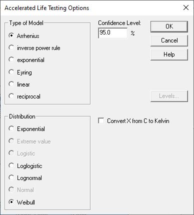
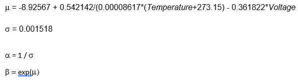
If the accelerating variable is temperature, the Arrhenius model is often used, which takes the following form:

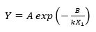
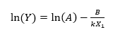
where Y is the failure time, X₁ is temperature in degrees Kelvin (°C + 273.15), k = 0.00008617 (Boltzmann’s constant), and A and B are two unknown parameters. Taking logarithms of both sides shows that the log failure time is linearly related to the reciprocal of temperature:

Additional accelerating factors such as voltage may be introduced by adding additional terms to the above equation. 

SAMPLE DATA

An an example, consider the data shown below:

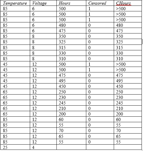
Data were collected at Temperature = 45, 65, and 85 degrees centigrade and at Voltage = 6, 8 and 12 volts. Hours represents either the time until each item failed or 500 if the item had not failed after 500 hours. Censored is set to 0 for actual failure times or to 1 if an item did not fail by 500 hours. An additional column named CHours is also shown, which is a special censored numeric data column. In that column, right-censored values are represented by the notation >500.

The goal of the study is to estimate the failure time distribution at normal operating conditions where Temperature = 25 and Voltage = 4. Note that these values have been added at the bottom of the datasheet, with the cell for Hours left empty. The Statgraphics ALT (Accelerated Life Testing) procedure will automatically recognize that combination of factors as one for which predictions are desired.

Data Input Dialog Box

The ALT data input dialog box takes the following form:

The Dependent Variable is a sample of individual failure times. It may be either:

1. a normal numeric column. In such cases, the Censoring field is used to indicate whether or not the row represents an uncensored failure time (indicated by entering a 0), a right-censored time (indicated by entering a 1), or a left-censored time (indicated by entering a -1).

2. a special censored numeric column. In such cases, the Dependent Variable field is used to indicate whether or not the row represents an uncensored failure time (indicated by entering a number such as 475), a right-censored time (indicated by entering an expression such as >500), a left-censored time (indicated by entering an expression such as <50), or an interval-censored observation (indicated by entering an expression such as [300,350]). The Censoring field is not used.

If multiple samples have the same characteristics, such as the first 3 rows of the data file shown above, the Sample Sizes field may be used to specify the number of samples represented by each row of the file.

The Quantitative Factors and Categorical Factors fields specify the predictor variables. There must be at least 1 quantitative factor, with the first factor entered considered to be the primary accelerating factor (Temperature in this case). As will be seen below, various acceleration models may be chosen for the primary factor. Other factors such as Voltage will be entered as linear terms in the regression model. If a reciprocal model is desired for other factors, enter them in the data input dialog box by entering expressions such as 1/Voltage.

Analysis Options

After specifying the input data, an Analysis Options dialog box will be displayed.

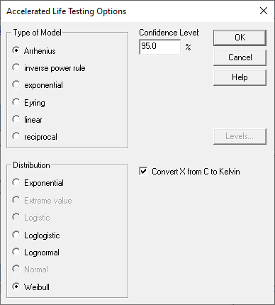
This dialog box is used is select the type of acceleration model for the primary factor. It is also used to select the distribution of failure times. Depending on the distribution selected, a number of parameters must be estimated. For example, the Weibull distribution has 2 parameters: a shape parameter and a scale parameter. The shape parameter is assumed to have a constant value which does not depend on the predictor variables. On the other hand, the value of the scale parameter changes as a function of the predictor variables. A typical Weibull distribution is shown below:

Analysis Summary

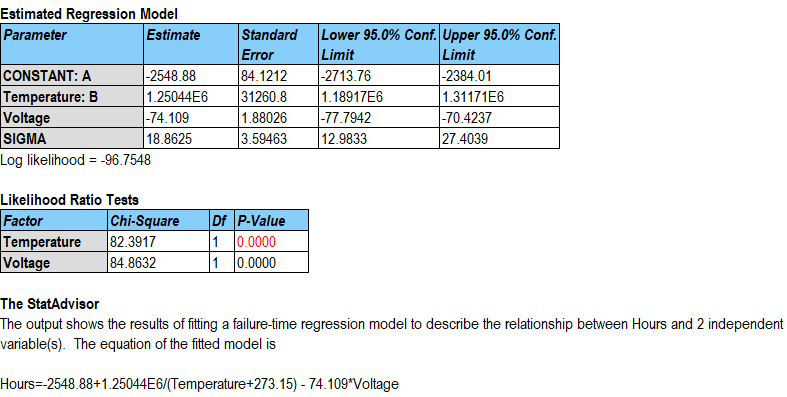
Fitting the requested model to the data generates an analysis summary that shows the fitted model. The summary for the sample data is shown below:

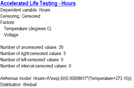
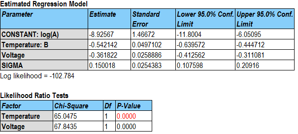
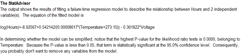
The estimated model for log(Hours) involves the reciprocal value of Temperature after converting it to degrees Kelvin and a linear function of Voltage. An increase in either predictor variable results in a lower prediction for log(Hours). An additional parameter sigma has also been estimated and is related to the dispersion of the failure time distribution.

Failure Time Distribution

The distribution of failure times for the sample data is assumed to follow a Weibull distribution, which has the following pdf:

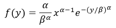
where a is the shape parameter and b is the scale parameter. For any combination of the predictor variables, the parameters may be determined by solving the following equations:

It may be seen that the scale parameter is a function of the predictor variables but the shape parameter is not. The shape parameter is only related to s.

Similar equations may be derived for the other distributions.

Model Verification

Before accepting the results of an accelerated life test, it is important to examine how well the selected model and the failure time distribution fit the observed data. Two plots are useful for this purpose. The first shows a plot of the observed failure times (excluding any censored data) predicted by the selected model. The plot for the sample data is shown below:

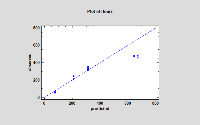
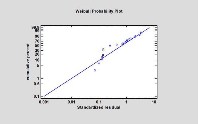
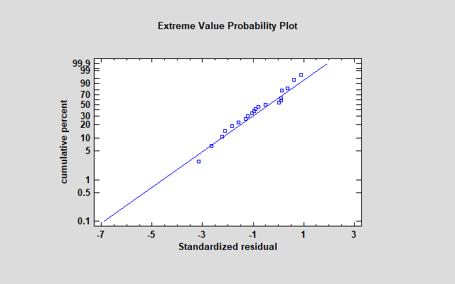
The deviation of the predictions from the diagonal line at large values of hours suggests that the model is overpredicting time to failure for the highest observed values. A residual probability plot based on the Weibull distribution shows that the data are not well predicted by that distribution, since the points deviate significantly from a diagonal line:

Experimenting with other models shows much better results using a reciprocal model with an extreme value failure time distribution:

Again, both of the predictor variables are highly significant:

The smallest extreme value distribution is defined by 2 parameters: the mode and a scale parameter. The mode is equal to the value m generated by the fitted equation while the scale parameter equals s.

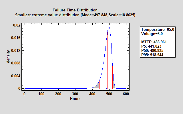
The failure time distribution shown above is much tighter than the earlier Weibull distribution.

Extrapolation

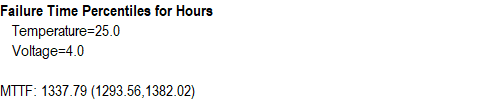
To estimate the failure time distribution at the normal operating conditions where Temperature = 25 and Voltage = 4, the equations shown above may be used to estimate the failure time distribution as shown below:

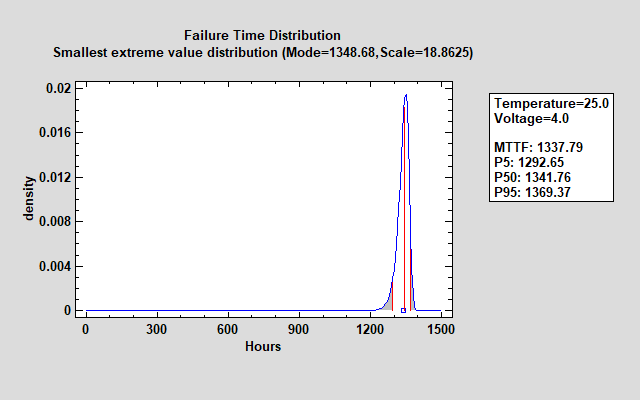
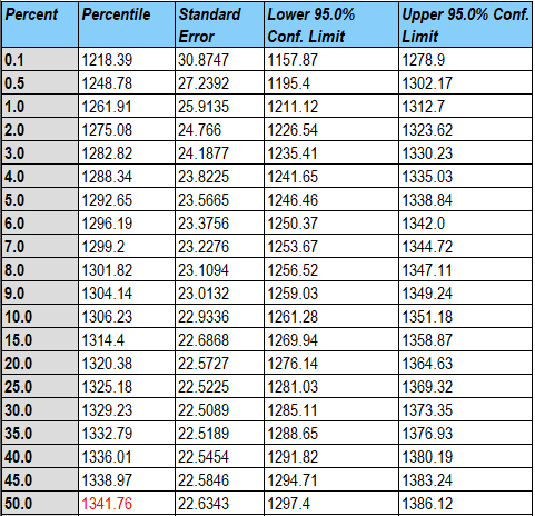
The mean time to failure (MTTF) at that combination of the predictor variables is estimated to be slightly more than 1,300 hours. 90% of the distribution lies between approximately 1,292 and 1,369 hours as indicated by the estimated percentiles.

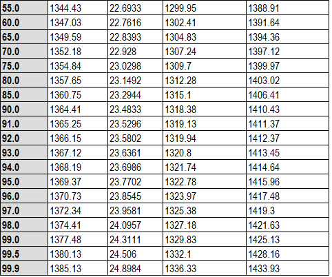
Confidence limits may also be calculated for the percentiles and the mean time to failure.

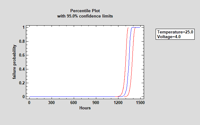
The percentiles and confidence limits may also be displayed graphically.

Conclusion

Accelerated life tests can provide an estimate of a failure time distribution at combinations of stress factors where experimentation is not practical. Obviously, the results depend on the acceleration model selected and the assumed failure time distribution. Where possible, those decisions should be made after looking at the published results of similar studies and verified by examining the current data.