

 By:
By: Published under: new feature, statistical analysis, data analysis, Data analytics, Predictive analytics, Titanic, Regression, Statgraphics, Multivariate methods, analytics software, machine learning, Statgraphics 18, classification, data mining, decision trees
The Classification and Regression Trees procedure added to Statgraphics 18 implements a machine-learning process that may be used to predict observations from data. It creates models of 2 forms:
- Classification models that divide observations into groups based on their observed characteristics.
- Regression models that predict the value of a dependent variable.
The procedure begins with a set of possible predictor variables, some of which may be categorical and others that are continuous. The models are constructed by creating a tree, each node of which corresponds to a binary decision. Given a particular multivariate observation, one travels down the branches of the tree until a terminating leaf is found. Each leaf of the tree is associated with a predicted class or value.
As an example, consider the data shown below listing all passengers who were onboard the Titanic on the night that she struck an iceberg and sank:
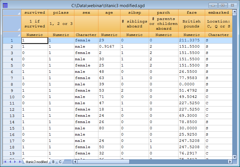
The data contain information on 1,309 passengers. A classification tree could be created to predict whether each individual survived or not based on his or her age, gender, class of ticket, etc. In addition to a binary decision (survived or not), the tree could also be used to estimate the probability that an individual with various characteristics survived.
Training, Validation and Prediction Sets
When using a machine learning algorithm like Classification and Regression Trees, observations are typically divided into three sets:
- A training set which is used to construct the tree.
- A validation set for which the actual classification or value is known, which can be used to validate the model.
- A prediction set for which the actual classification or value is not known but for which predictions are desired.
In Statgraphics 18, this procedure automatically puts all observations for which the output variable is missing into the third set. The rest of the observations are divided between the first 2 sets according to the option selected on the Analysis Options dialog box:
Putting every other row into the training set and the others into the validation set is often a reasonable approach.
Recursive Partitioning
Constructing a classification or regression tree involves successively partitioning the data into more and more groups based on the value of a predictor variable. The first partition takes the entire training set and divides it into 2 groups. Each group is then further divided into 2 subgroups and each of those subgroups is divided again. Partitioning the data into subgroups continues until all of the observations in a particular subgroup are the same or until some other criterion is met.
When deciding how to partition a group of observations, binary decisions involving each predictor variable are considered. A typical partition based on a categorical factor might involve answering the question "Is sex equal to female?" A typical partition based on a quantitative factor might involve answering the question "Is age less than 50?" The partition selected is the one which minimizes the residual mean deviance. For a regression tree, the residual mean deviance is defined by
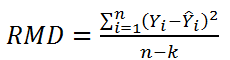 where Yi is the i-th observed value of the dependent variable,
 ![]() is the predicted value for the subgroup to which it is assigned, n = the total number of observations in the training set, and k is the total number of subgroups (leaves) in the tree. The predicted value of each subgroup is the average value of Y for all observations in the training set assigned to that subgroup. For a classification tree, the residual mean deviance is defined by
is the predicted value for the subgroup to which it is assigned, n = the total number of observations in the training set, and k is the total number of subgroups (leaves) in the tree. The predicted value of each subgroup is the average value of Y for all observations in the training set assigned to that subgroup. For a classification tree, the residual mean deviance is defined by
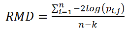
where pi,j is the estimated probability that observation i would be assigned to class j and j is the class predicted by the model.
To understand the concept of residual mean deviance for classification models, consider the following mosaic chart:
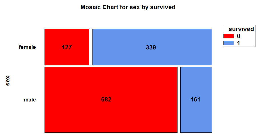
This chart shows a breakdown of the 1,309 passengers on board the Titanic by sex and whether or not they survived. Of the 466 females on board, 339 survived while 127 did not. Of the 843 males on board, 161 survived while 682 did not. Based on sex alone, a classification model would predict that a female would survive while a male would not. The residual mean deviance equals
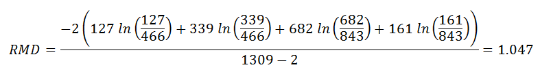
The better the binary choice discriminates between the classes, the lower the value of RMD.
Decision Trees
In Statgraphics 18, a decision tree is created by selecting R Interface - Classification and Regression Trees from the main menu. For the Titanic dataset, the data input dialog box should be completed as shown below:
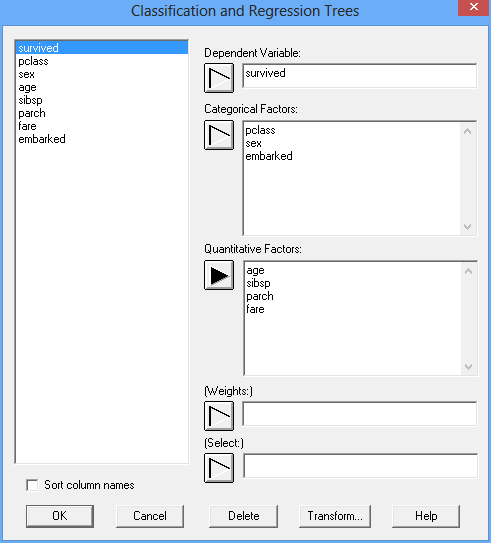
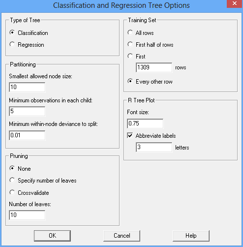
A classification model is to be constructed to predict the value of survived using 3 categorical factors and 4 quantitative factors. Partitioning is controlled by the Analysis Options dialog box:
Note the following settings:
1. Type of Tree: This has been set to Classification so that the model will predict either a 0 or a 1 for survived. If set to Regression, survived would be considered to be a continuous variable.
2. Partitioning: These settings control how extensively the subgroups will be partitioned. Based on the options shown above, subgroups will be considered for partitioning only if they have at least 10 members. Also, the only partitions that will be considered are those for which each child (subgroup) has at least 5 members. In addition, no subgroup will be partitioned if the deviance within that subgroup is less than 0.01.
3. Pruning: Once a tree has been constructed, it may be pruned by removing branches. Pruning will be discussed more below.
4. Training set: All rows will be placed in the training set and used to build the tree.
The resulting tree is shown below:
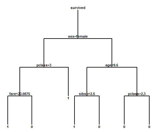
To classify an individual, begin at the top of the tree. At the decision point labeled "sex=female", move left if that statement is true or right if it is not. For a female passenger, move left to the decision point "pclass=3". If the person has a first or second class ticket, move right to the leaf labeled "1" which predicts that the individual will have survived. If the person has a third class ticket, move to the decision point "fare<23.0875". At this point, individuals with less expensive tickets move left and are predicted to have survived. Individuals with more expensive tickets move right and are predicted not to have survived!
Node Probabilities
Examining the decision tree shown above, it will be noticed in the lower right corner that both branches following the decision point "pclass=2,3" lead to a prediction of 0 for survived. While the predicted survival may be the same along each branch, the probability of survival is not. For a classification tree, it is useful to examine the probability distribution at each leaf of the tree. Statgraphics 18 shows this through a table of node probabilities:
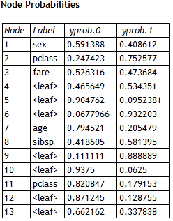
The table shows the proportion of observations in the training set that arrived at each node (decision point or leaf) and belonged to the classes survived=0 and survived=1. Leaves 12 and 13 are the leaves in the lower right corner of the tree. Of all males more than 9.5 years old, about 34% survived if they had a first class ticket while only 13% survived if they had a second or third class ticket.
Pruning
Once a tree has been constructed, it is frequently of interest to prune it (remove branches). This can be helpful when the data have been overfit, a phenomenon where a complicated tree is created which fits the training data well but is too complex for predicting other cases well. The Analysis Options dialog box shown earlier offers 2 options for pruning:
1. Specify number of leaves: The tree will be pruned back to one with a specific number of leaves by removing those branches which contribute the least to the reduction of the residual mean deviance.
2. Crossvalidate: A cross-validation experiment will be performed to find the deviance as a function of the number of leaves in the tree.
The crossvalidate option will find the best tree with 1 leaf, the best tree with 2 leaves, the best tree with 3 leaves, up to the number of leaves specified. It results in a plot similar to that shown below:
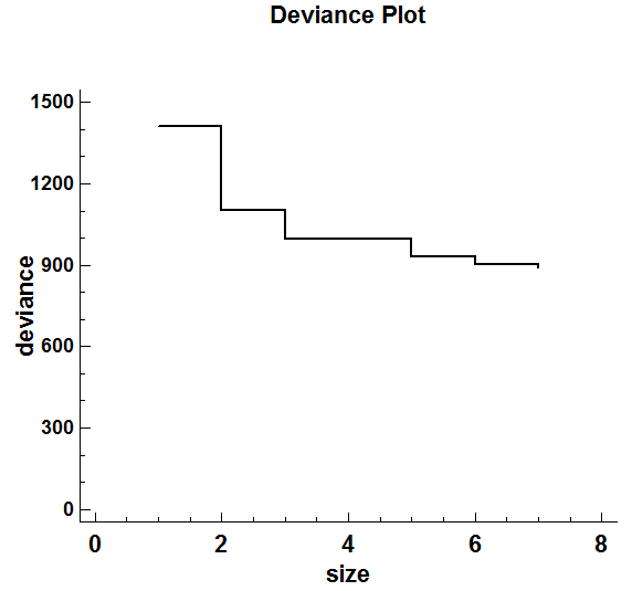
This plot indicates the total deviance for each size tree. Note that adding the 6th and 7th leaves results in a very small reduction. Pruning the tree back to 5 leaves gives the following tree:
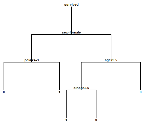
Interpretation of the tree is now much simpler. The only passengers that would be predicted to have survived are females with first and second class tickets and males less than 9.5 years of age with 2 siblings or less onboard.
Using a Validation Set
Let's redo the tree fitting process by dividing the 1,309 passengers into a training set and a validation set. Using the "every other row" option on the Analysis Options dialog box to create the training set results in a slightly different tree:
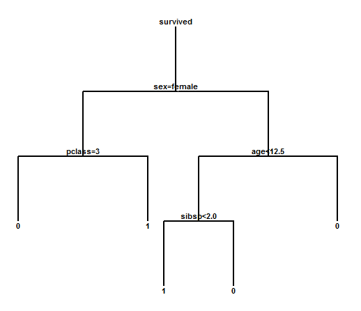
It's basically the same tree but some of the splitpoints are slightly different. To compare the results of the training set and validation set, Statgraphics 18 constructs the following table:
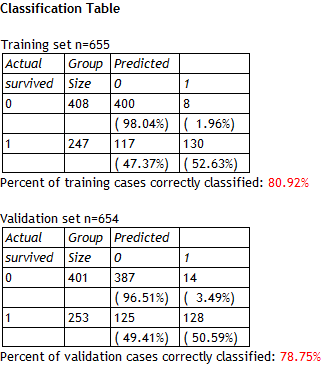
The model correctly predicted survival for approximately 81% of the 655 individuals in the training set and approximately 79% of the 654 individuals in the validation set. Such a small degradation of performance in the validation set is a very good sign that the model is working well. Notice also that the model was very good at predicting those individuals that did not survive but not as good at predicting those that did survive.
Missing Data
As with most statistical procedures, special attention must be given to data with missing values. In the Titanic dataset, the age of 263 of the 1,309 passengers was not known. Also, the data is missing for 1 passenger's fare and 2 passengers' embarkation point. The procedure used by Statgraphics 18 handles missing data in the following way:
1. Any cases in the training set that have missing data for any of the predictor variables are not used to fit the tree.
2. When predicting cases for comparison of the validation and training sets, individual cases travel down the tree as far as possible before hitting a decision point at which the required variable is missing. The node probabilities at that decision point are then used to make a prediction for that case. For example, in the trees shown above males of unknown age move only as far as the decision point "age<12.5". Since a majority of observations in the training set that make it to that node did not survive, those of unknown age would also be predicted to not survive.
Regression Trees
The major difference between a classification tree and a regression tree is the nature of the variable to be predicted. In a regression tree, the variable is continuous rather than categorical. At each node of the tree, predictions are made by averaging the value of all observations that make it to that node rather than tabulating proportions.
Any interesting dataset for illustrating a regression tree is shown below:
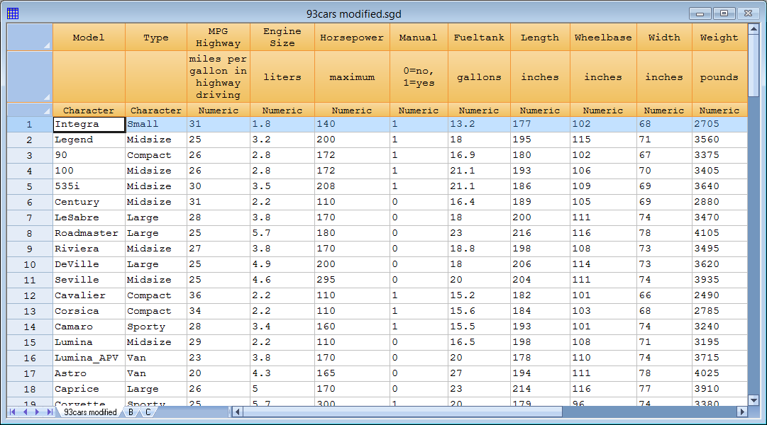
The datasheet shows data for 93 makes and models of automobiles. To develop a regression tree for predicting MPG Highway, select R Interface - Classification and Regression Trees and complete the data input dialog box as shown below:
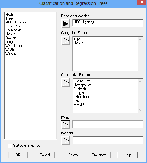
Be sure to select Regression tree on the Analysis Options dialog box:
After creating a tree and pruning it back to 7 leaves, its diagram is shown below:
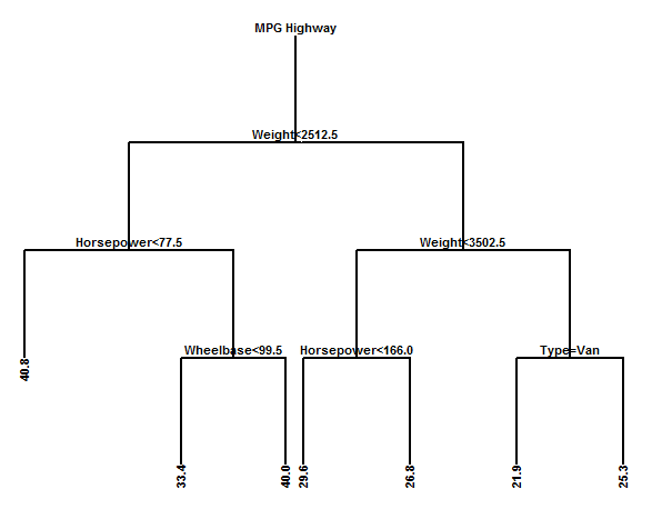
The highest predicted miles per gallon in highway driving is not surprisingly associated with light cars with low horsepower. The lowest predicted miles per gallon is for heavy vans.
The one additional plot that should be examined for regression trees is a plot of the residuals versus predicted values:
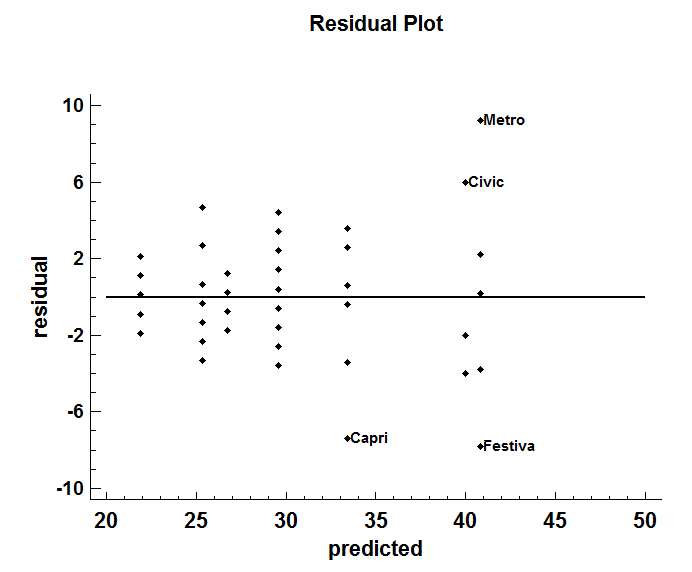
There are 4 cars with residuals greater than 6 in absolute value. In addition, note some possible increase in variability with increasing predicted miles per gallon.
References
Brieman, L., Friedman, J., Stone, C.J. and Olshen, R.A. (1998) Classification and Regression Trees. Wadsworth.
(2015) Data Mining with Decision Trees: Theory and Applications, 2nd edition. World Scientific.
Zhang, H. and Singer, B.H. (2010) Recursive Partitioning and Applications. Springer.


