

 By:
By: Published under: bivariate density, statistical analysis, data analysis, R, Cluster analysis, machine learning, distribution fitting
When modeling a set of data that has more than one mode, simple distributions are not sufficient. Instead, it may be necessary to fit a mixture of more than one distribution. For example, the data below display the duration of 272 consecutive eruptions of the Old Faithful geyser in Yellowstone National Park:
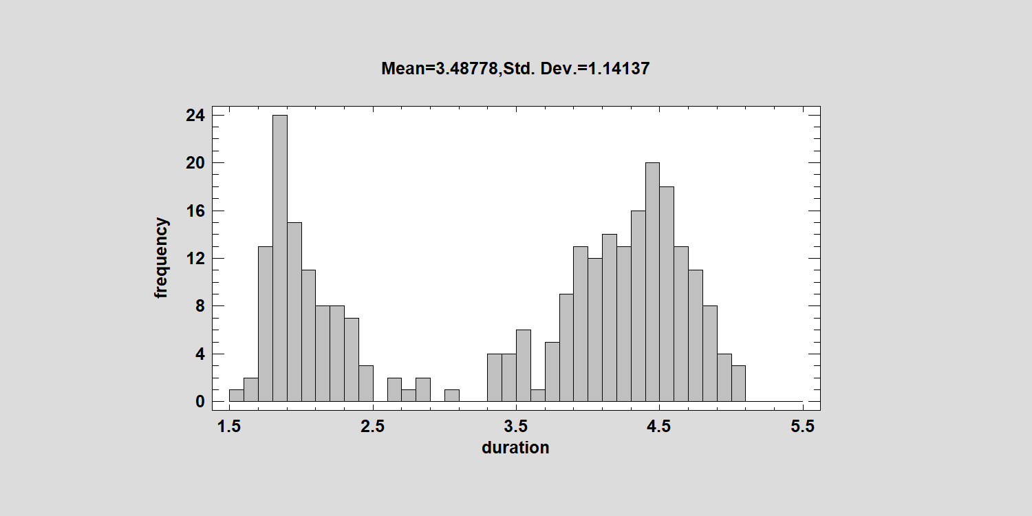
There appear to be 2 well-defined peaks: one near 2 minutes and the other close to 4.5 minutes. While one might question whether these 2 components are normally distributed, it is instructive to attempt to model them using a mixture of normal distributions.
In general, a mixture of K normal distributions may be represented by
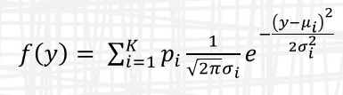
which is parameterized by K means, K standard deviations, and K proportions where
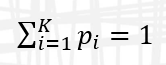
Statgraphics 19 includes an interface to the EMCluster package in R. If we ask the program to fit a mixture of 2 components, we observe the following:
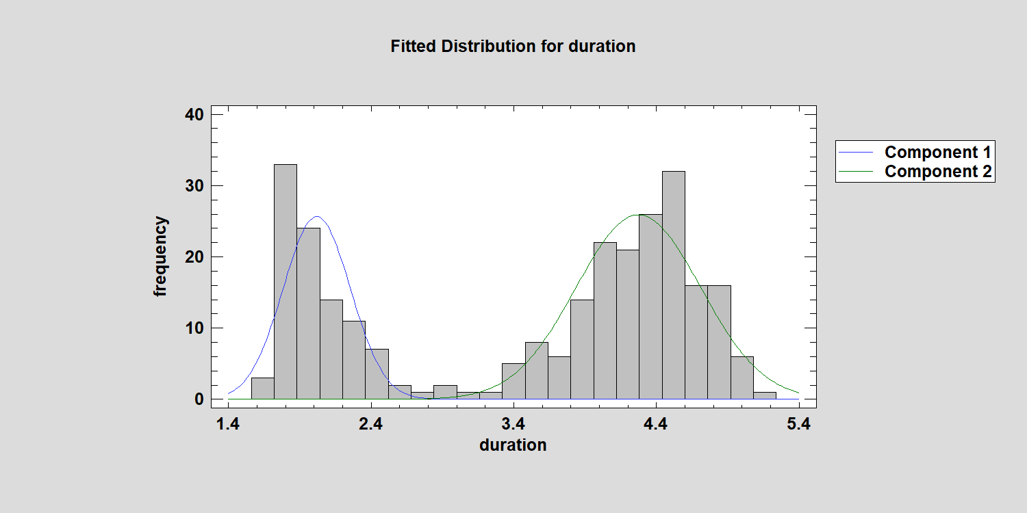
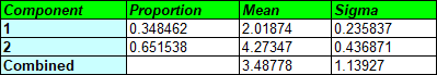 This table shows that about 35% of all eruptions are represented by a component with a mean of 2.02 minutes, while the other 65% are represented by a component with a mean of 4.27 minutes.
We can test the goodness-of-fit by running a chi-squared test, which compares the observed number of data values in adjacent intervals with the number expected for the fitted distribution: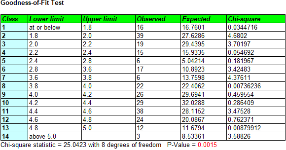
The small P-Value confirms our suspicions that the data are not well modeled by a mixture of Gaussian distributions.
That leaves us with two choices:
- Try fitting the data with a mixture of more than 2 Gaussian components.
- Try a mixture of 2 or more non-normal distributions.
Since the EMCluster package in R only handles Gaussian mixtures, I tried fitting a mixture of 4 normal distributions. This is what I got:
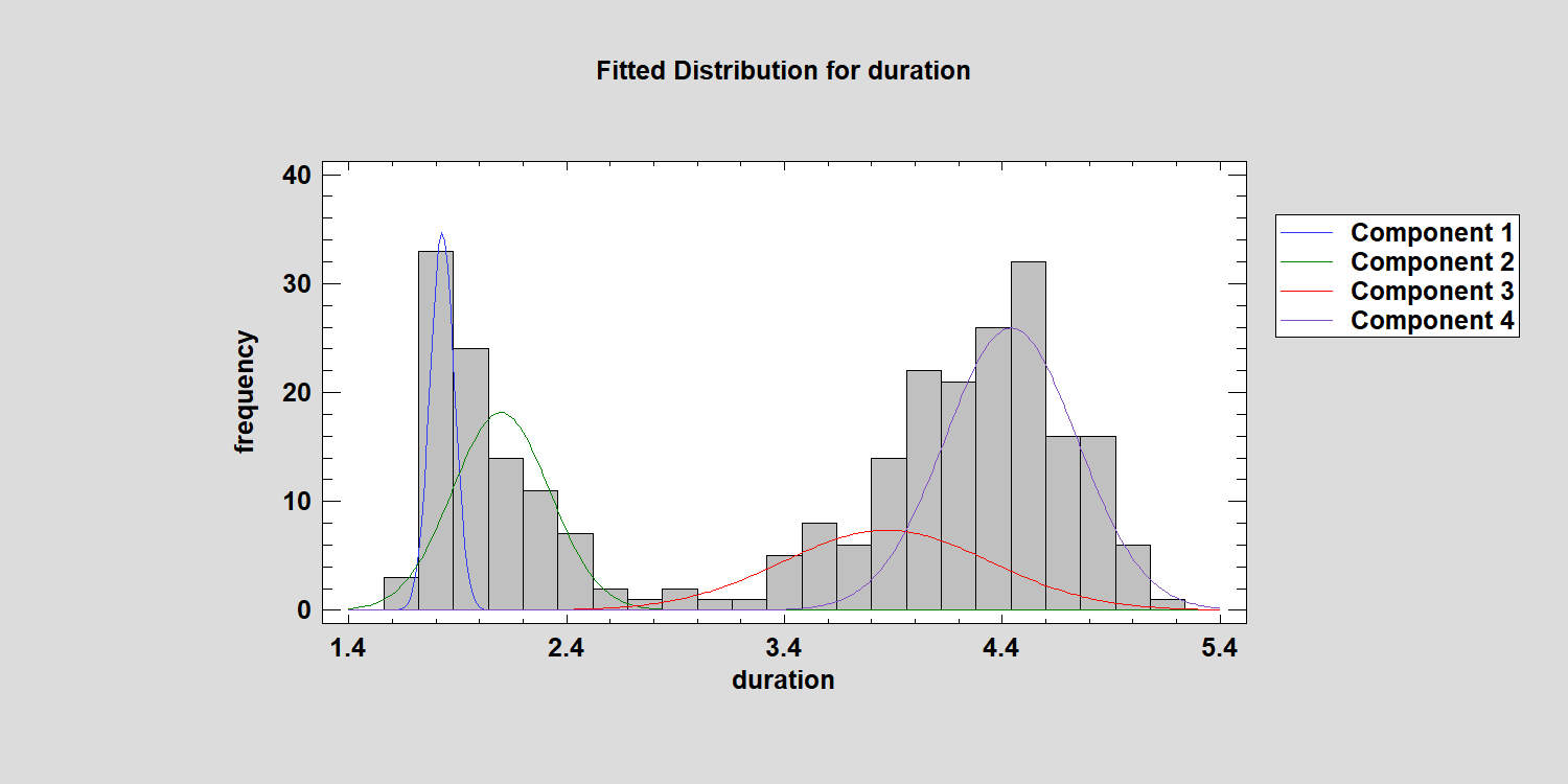
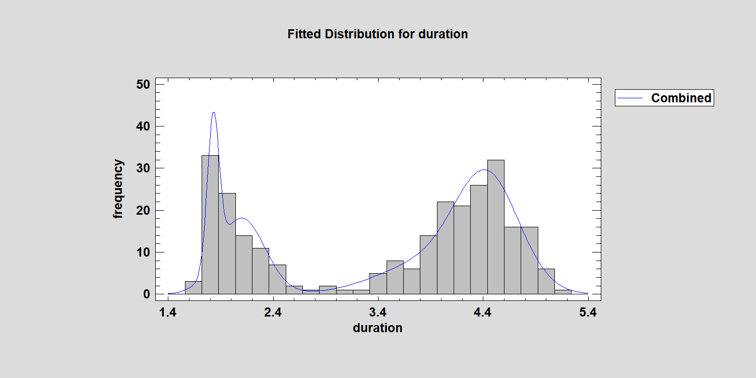
A four distribution mixture appears to be a better fit, but the P-Value is still only around 0.02. By the way, the combined distribution is a little funky:
Statgraphics 19 generates a table that we may use to compare models with different numbers of components:
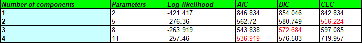
It includes the Akaike Information Criterion (AIC), the Bayesian Information Criterion (BIC), and the Classification Likelihood Criterion (CLC). In each case, smaller values indicate a better fit. There is obviously some disagreement, but that might depend on what we intend to do with the model. I read recently that the BIC is a very good criterion to use when the components are in fact Gaussian, but may overestimate the number of components in the data when non-normality is present. That might be okay if my primary interest is estimating the probability density function. But if my primary interest is dividing the data into groups, then the CLC may be better. Of course, we could also try estimating a mixture of non-normal distributions. I recently found another package in R which can fit mixtures of normal, lognormal, gamma and Weibull distributions. We're in the process of adding an interface to that package and will report back once that's complete.
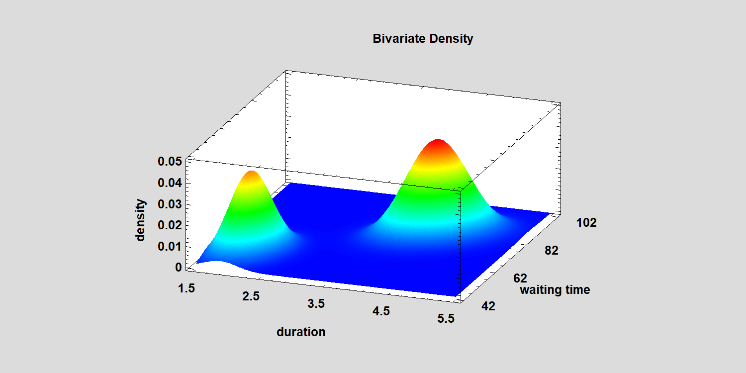
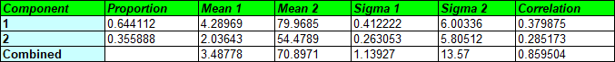
It's also possible to fit a mixture of bivariate Gaussian distributions when you have 2 correlated variables. The plot below shows a 2-component mixture fitted to the duration of the Old Faithful eruptions and the waiting time until the next eruption:
It turns out that after a short eruption, the mean waiting time until the next eruption is approximately 54.5 minutes, while the mean waiting time after a long eruption is about 80 minutes:
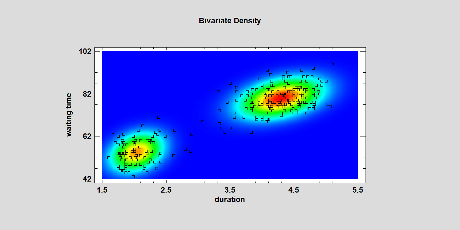
For purposes of clustering, this model works very well:
One last comment: selecting a proper model is important. There's always a danger in overfitting data. A complicated model begins to model not just the underlying reproducible patterns but also some of the noise specific to the sample used to fit the model. If one's goal is predicting other data sets, it's best to keep the models as simple as possible.
If you'd like more details on these examples, view our recorded webinar:


