Version 20 of Statgraphics Centurion adds 10 new supervised machine learning (ML) procedures to its collection of methods for predictive analytics. Supervised ML procedures are AI algorithms that use a set of data with known outcomes to predict cases where the outcome has not yet been determined. The algorithms are fit to a training dataset and tuned using either a set of known cases in a separate test set or using cross-validation performed on the training set. The ML procedures handle 2 types of outcomes: categorical outcomes where one or more input features are used to classify each case, or quantitative outcomes where the input features are used to predict the value of the outcome variable.

Version 20 also contains a Supervised Machine Learning Wizard which makes it easy to apply multiple methods to the same dataset. The wizard also allows multiple methods to be combined to create a single ensemble prediction.

Example

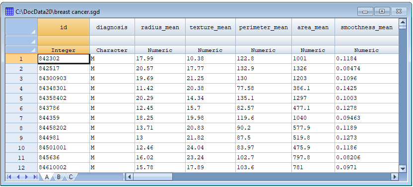
The UC Irvine Machine Learning Repository (https://archive.ics.uci.edu/) contains a data set collected at the University of Wisconsin with information on 569 masses found in women's breasts. Each mass is characterized by 30 measurements made on the cell nuclei in a digitized image taken using a fine needle aspirate (FNA). Each mass was later determined to be either malignant or benign. The goal is to classify unknown masses as malignant or benign based on the 30 measurements. Part of the file is shown below:

Supervised Machine Learning Wizard

In Version 20, users have a choice of running the 10 new machine learning procedures separately or under the control of a wizard. The wizard has several advantages:

1. The input data needs to be specified only once regardless of how many methods are used.

2. The predictive ability of multiple procedures is compared side-by-side in both tabular and graphical formats.

3. Multiple methods may be combined to produce a single ensemble prediction that may be better than using only a single method by itself.

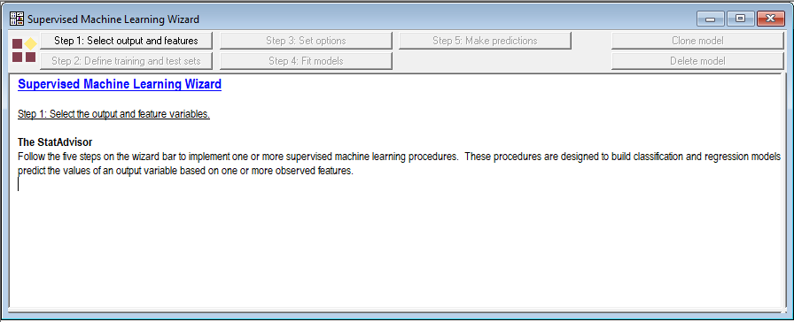
To run the wizard, the user goes to the Learn menu and selects Wizard (Python). Each of the procedures called by the wizard is contained in the Python library named scikit-learn (https://scikit-learn.org/stable/index.html). The wizard brings up a window with a toolbar that guides the user through 5 steps of model-fitting and prediction:

Step 1: Select output and features

Each ML procedure expects one output variable and one or more input variables containing features that could be used to predict the outcome:

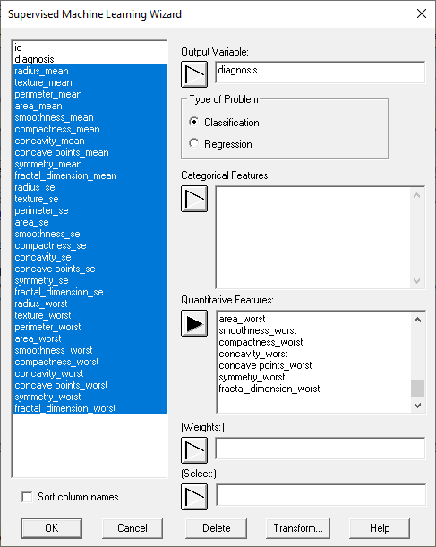
The user also specifies whether this is a classification or regression problem. Weights may be specified if some cases are to be given more weight than others. This is especially helpful when each row of the data file represents a group of subjects rather than an individual subject. In such cases, the weights are usually set equal to the group sizes.

Step 2: Define training and test sets

In supervised machine learning, the cases in the data file are usually divided into 3 sets:

Set #1: a training set with known outcomes that is used to train or fit the algorithm.

Set #2: a test set with known outcomes that is not used during training. Predictions made on the test set are used to determine how well a method performs and to select between different methods.

Set #3: a prediction set with unknown outcomes for which predictions are made once the method has been trained. 

The wizard displays the following dialog box to assist users in defining these sets:

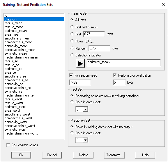
The dialog box above puts all of the rows in the training set since the sample size is relatively small.

Note that it is not necessary to define a test set. Instead, all cases with known outcomes can be placed in the training set, which is helpful when the number of cases is small. In the absence of a test set, validation of the method relies on cross-validation. The most common type of cross-validation is 5-fold cross-validation, where the training set is divided into 5 subsets. The method is then applied 5 times, each time holding back 20% of the cases in the training set. Statistics are then calculated on how well the method can predict the cases that were not among the 80% of the cases used to train each model. Results of the 5 "folds" are then averaged to determine the algorithm's performance.

Step 3: Set options

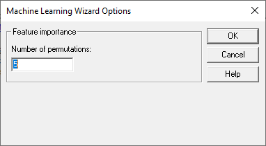
When a large number of features are used by an algorithm, it typically happens that some features are more important in predicting the outcome than others. To determine which features are most important, ML algorithms often check how important each feature is by randomly permuting the entries in a selected feature column and assessing how much worse the predictions are than using the true sequence of feature values. The more important a feature, the greater the difference between how well the method performs when the values in that column are in their proper order compared to how well it performs when the values are randomly shuffled. 

The dialog box for Step 3 specifies how many times each feature column should be permuted:

Step 4: Fit models

The Step 4 button is used to train one or more algorithms. It displays the following dialog box:

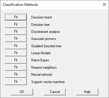
Each time one of the Fit buttons is pushed, the indicated procedure is invoked. Note that the same procedure can be selected more than once. since users might want to try running the same procedure with different parameter settings.

Suppose for example the Nearest neighbors button is selected. Before training the model, the Analysis Options dialog box for that procedure will be displayed:

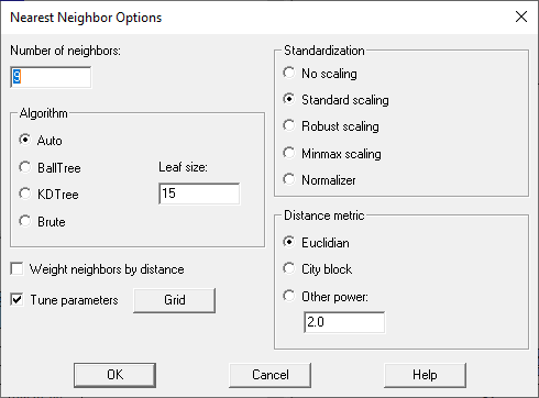
Conceptually, the nearest neighbors procedure predicts an unknown case by matching it to a specified number of training cases (5 by default) that are closest to the unknown case in the space of the feature variables. Users have various choices:

1. the number of nearest neighbors to match each case to.

2. the algorithm used to find the nearest neighbors (in large data sets, it is very time-consuming to try all possibilities).

3. how feature variables, which often have different units, should be scaled before calculating distances.

4. how distance should be calculated.

5. in making a prediction, whether more weight should be given to the closest neighbors.

Obviously, there are many combinations of the parameters that could be selected. To help users find good parameters values, each Analysis Options dialog box has a checkbox labeled Tune parameters and a button labeled Grid. If selected, the algorithm will be trained using various combinations of parameter values specified by the dialog box displayed when the Grid button is pressed:

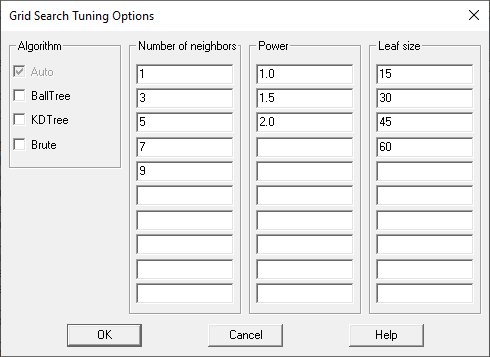
By default, the nearest neighbor method will be trained 60 times (1 algorithm with 5 numbers of neighbors with 3 values of power and 4 values of leaf size). Whichever combination gives the best predictive performance during cross-validation will be the combination selected.

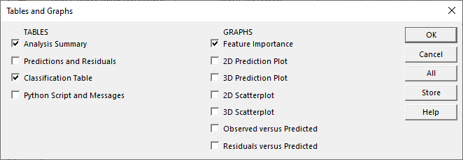
The user may also select various tables and graphs to display the results of the nearest neighbor method:

When OK is pressed, a new window will open and the results will be displayed:

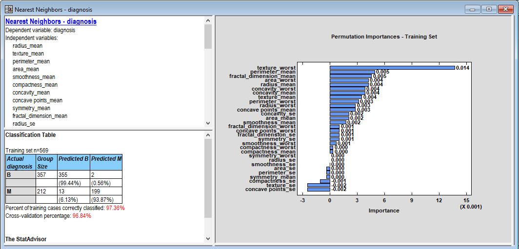
Of particular importance is the classification table in the lower left pane. The statistic used to assess how well a classification model performs is the percentage of cases that were correctly predicted. For the 569 cases in the training set, the nearest neighbor method was correct 97.36% of the time. It did slightly worse during cross-validation, with only 96.84% of the cases correctly predicted on average. Note that the rate of false positives (predicting that a benign tumor is malignant) is much lower than the rate of false negatives (predicting that a malignant tumor is benign). That's not a particularly good result if this method is to be used for screening. Interestingly, the grid search found the optimal number of neighbors to use when making a prediction is 9.

The feature importance plot in the right pane shows the 30 features plotted in decreasing order of importance. Here importance is measured as the increase in the proportion of correct predictions generated by ordering a feature in its proper order versus ordering it in a random order. The most important feature, texture_worst, generates about 1.4% higher correct predictions when ordered properly. 

If the Step 4 button is repeated for each method, the wizard will generate a chart comparing their performance:

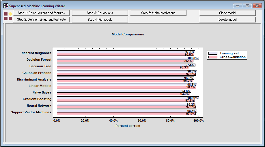
The best performing method during cross-validation was actually the Linear Models (a logistic regression in this case since the outcome is categorical). It was correct 98.1% of the time on average during cross-validation.

Step 5: Make predictions

The purpose of selecting and tuning one or more supervised machine learning procedures is usually to make predictions about cases where the outcome is not known. As an example, I added an additional row to the bottom of the data file in which I put the mean value of each feature but left the outcome blank. Rows without an outcome are automatically added to the prediction set.

During this step, the wizard first displays a list of all the methods that have been tuned.

.

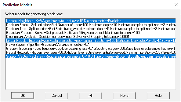
The user then selects one or more methods to use to predict unknown cases. It is sometimes helpful to select more than one method, which creates something called an ensemble prediction. If more than 1 method is selected, the wizard will then display a dialog box with options for combining predictions from the different methods:

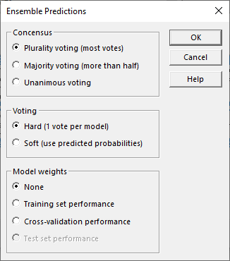
If desired, methods with better performance can be given more weight in determining the final prediction. Votes can also be combined based on the estimated probability that each method's prediction will be correct.

 When I gave each method 1 vote, the wizard generated the following output:

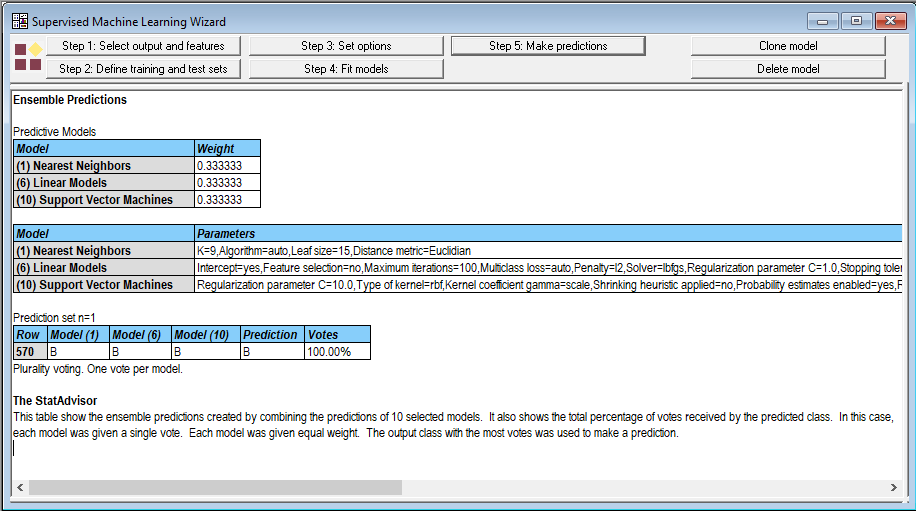
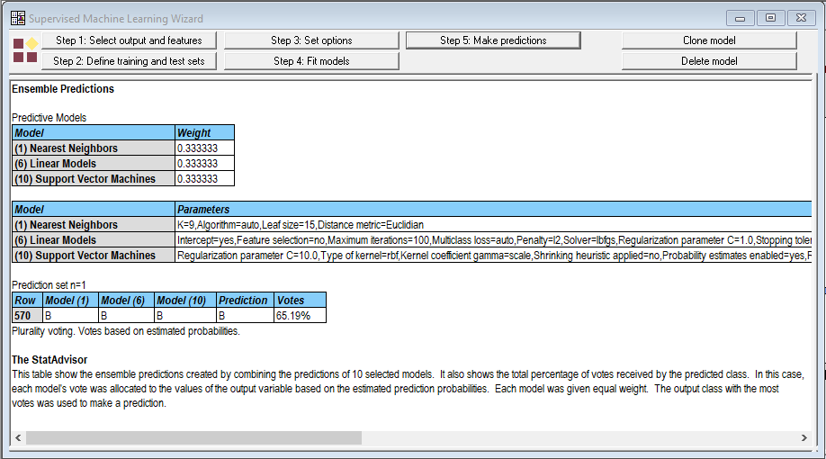
All 3 methods predicted that the mass would be benign. But when I selected the option to use predicted probabilities for voting, the results were not as encouraging:

Looking at the individual windows, I noted the following predictions:

Nearest neighbor:

Linear model:

Support vector machines:

The probabilities that the mass is benign average 0.6519 which was used to create the final vote. Not a result you'd want to bet your life on.