Chapter 7 of my newly published book Process Capability Analysis: Estimating Quality (CRC Press, 2018) deals with multivariate statistical process control, including multivariate statistical tolerance limits. Statistical tolerance limits have many important applications, particularly in the area of process capability analysis. Based on a sample of n observations taken from a population, they provide a region containing P% of the true population with C% confidence. For example, 300 observations might be sampled from the population and used to create an interval containing 99% of the population with 95% confidence.

For a single variable randomly sampled from a population characterized by a normal distribution, the statistical tolerance limits are calculated from the sample mean and sample standard deviation using the well-known formula

where k is a constant that depends on n, C and P. One-sided upper or lower bounds can also be constructed. Given specification limits for a product that range from a lower specification limit LSL to an upper specification limit USL, the calculated tolerance limits may be compared to the specification limits. If the tolerance interval is completely within the specification limits, then one may be C% confident that at least P% of the product will be in spec.

Univariate Tolerance Limits

As an example, consider the data shown below:

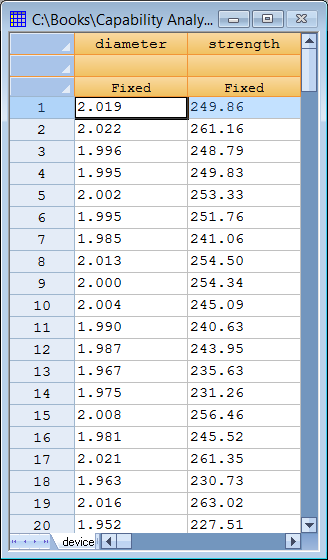
The table shows measurements made on the first 20 of 200 samples taken from a  manufacturing process. The specification limits for diameter are 2.0±0.1, while strength is required to be ≥ 200. The graph below shows a histogram of diameter for all n = 200 observations.

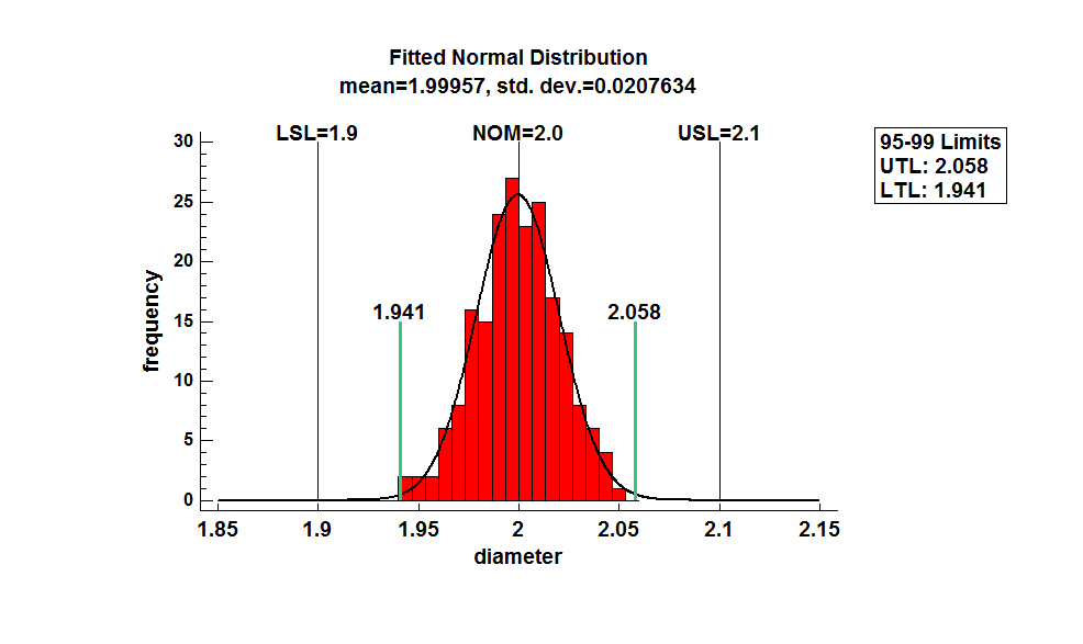
The graph shows the fitted normal distribution, the specification limits, and 95% statistical tolerance limits for 99% of the population (the green vertical lines). The entire tolerance interval [1.941,2.058] lies completely within the specification limits [1.9,2.1]. A similar plot for strength is shown below:

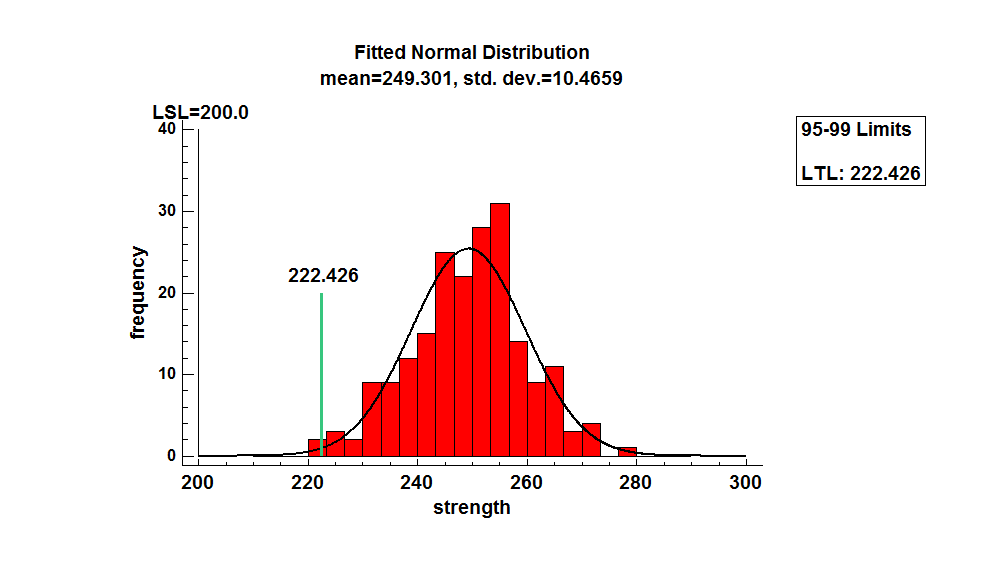
The 95% one-sided lower tolerance bound for 99% of the population of strength equals 222.426, which is well above the lower specification limit of 200.

Multivariate Normal Distribution

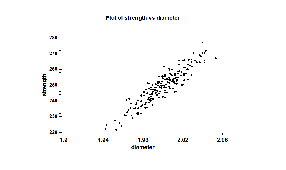
When more than one variable is collected, calculating separate tolerance limits for each variable does not tell the whole story. The fact that the 95-99 statistical tolerance intervals for both variables meet the specifications does not guarantee that both variables are SIMULTANEOUSLY within their specification limits 99% of the time. This is particularly true when the variables are correlated. For the sample data, the scatterplot below shows a strong positive correlation between diameter and strength:

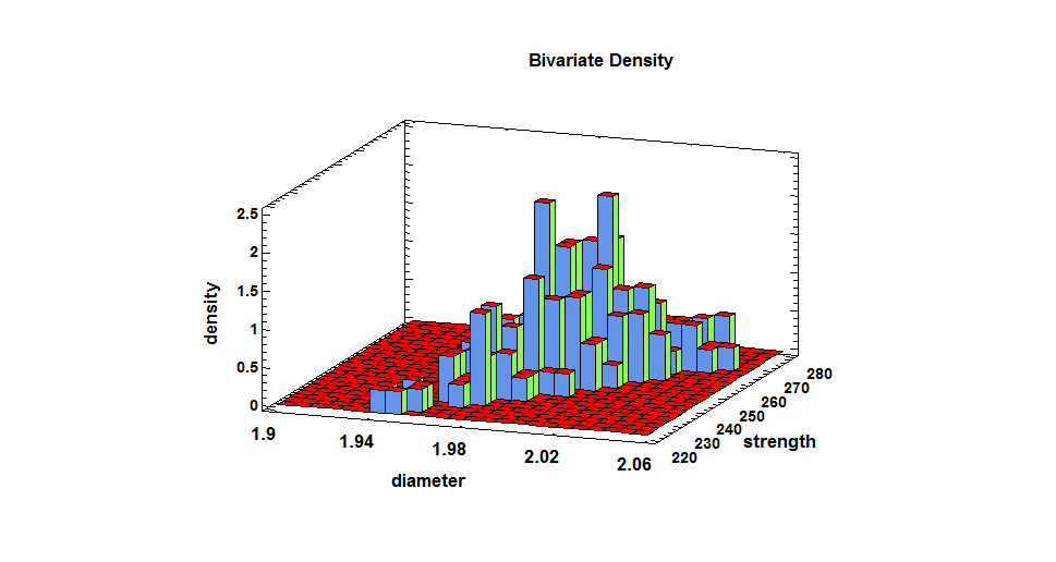
In such cases, it is important to use a multivariate approach to analyze the data. Plotting the data with a bivariate histogram shows a well-defined peak near the center of the data:

The most widely used model for multivariate data is the multivariate normal distribution. Given m variables, the distribution may be defined by a vector of m means, m standard deviations, and an m by m correlation matrix. It has the important property that any linear combination of the m variables (including each variable taken singly) has a univariate normal distribution. The graph below shows a bivariate normal distribution fitted to the n=200 bivariate observations of diameter and strength:

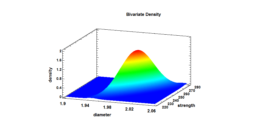
It has a well-defined peak and falls off symmetrically from that peak. When plotted as a 2-dimensional contour plot, it is possible to see the elliptical nature of the density function:

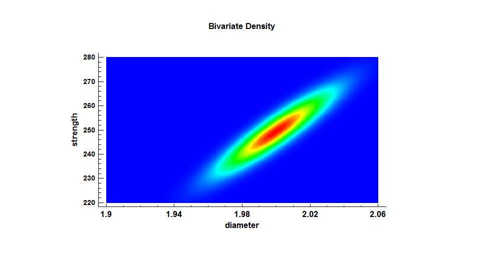
The elongation from bottom-left to top-right is caused by the positive correlation between the 2 variables.

Multivariate Tolerance Limits

Multivariate statistical tolerance limits may be calculated from n multivariate observations such that the limits bound P% of all items in the population with C% confidence. Assuming that the data are random samples from a multivariate normal distribution, this may be done in either of 2 ways:

1. Separate tolerance limits may be constructed for each variable, each of which bounds P% of the values of a selected variable with confidence level (C-100+100m)/m%. For example, if m=2 then each tolerance limit would be incorrect (100-C)/2% of the time. The true confidence level associated with the region defined jointly by the separate tolerance limits will be greater than or equal to C%.

2. An elliptical region may be constructed that bounds P% of the multivariate observations with exactly C% confidence. This region is defined by

where Y is an m by 1 multivariate random variable,  is the vector of sample means, S is the sample covariance matrix, and k is a constant that depends on m, n, P and C. The value of k is usually determined using Monte Carlo simulation, since it cannot be derived theoretically and there are no reliable approximations for it.

 The figure below shows multivariate statistical tolerance limits for 99% of the sample data with 95% confidence:

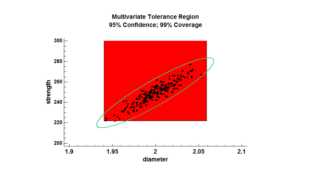
The rectangular region shows the simultaneous univariate limits for 99% of the population, each calculated with 97.5% confidence. The ellipse is an exact 95-99 multivariate tolerance region. Notice that the region defined the ellipse is much smaller than the rectangular region. Note also that each region contains some combinations of diameter and strength that are not contained in the other region.

Distance Plot

In 2 dimensions, it is easy to determine whether individual observations are within the elliptical region. In higher dimensions, it’s a more difficult task. A good tool for visualizing how extreme selected values are is to plot the squared standardized distances

 for i =1,2,…,n. Any values of d_i² > k are outside of the tolerance region. The plot below shows the squared distance with the critical value k = 10.664:

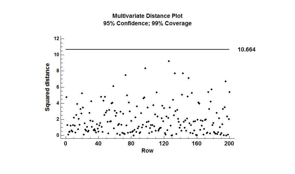
Since all of the 200 squared distances are less than k = 10.664, all of the bivariate observations lie within the 95-99 elliptical tolerance region.

Analyzing Multivariate Non-Normal Data

For data that do not follow a multivariate normal distribution, it may be possible to transform the data in such a way that the transformed values follow such a distribution. If so, the specification limits may be transformed in a similar manner and statistical tolerance regions calculated in the transformed metric. Andrews et al. (1971) proposed an approach for finding a multivariate transformation that parallels the Box-Cox procedure for univariate data. It assumes that there is a vector of powers λ= {λ₁, λ₂, …, λ_m) that when applied to the m variables transforms them to a metric in which they follow a multivariate normal distribution. Maximum likelihood estimates of the powers may be obtained by maximizing the profile likelihood function, which needs to done numerically.

A practical approach for dealing with multivariate data that may be non-normal is as follows:

Step 1: Perform Royston’s test for multivariate normality. In Statgraphics 18, this is located on the main menu under Describe – Multivariate Methods – Multivariate Normality Test. It gives output similar to that shown below:

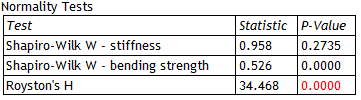
The output shows the result of running the Shapiro-Wilk test on each variable separately and Roysten’s test for multivariate normality. A small P-Value (less than 0.05) for Roysten’s test leads to rejection of the hypothesis that the data come from a multivariate normal distribution.

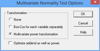
Step 2: If the multivariate normal distribution is rejected, determine the best multivariate power transformation. This may be done within the same procedure used in Step 1 by selecting Analysis Options and setting the options as shown below:

As in the Box-Cox transformation, a value called an “addend” may be added to each observation before applying the power transformation. The optimal transformation will be displayed:

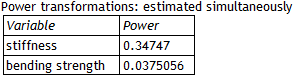
In this case, the optimal transformation is very close to a cube root for stiffness and a logarithm for bending strength. Roysten’s test may then be applied to the transformed data to determine whether a multivariate normal distribution is appropriate for the transformed data:

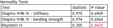
The large P-Value indicates that the procedure successfully determined a metric in which the data are well represented by a multivariate normal distribution.

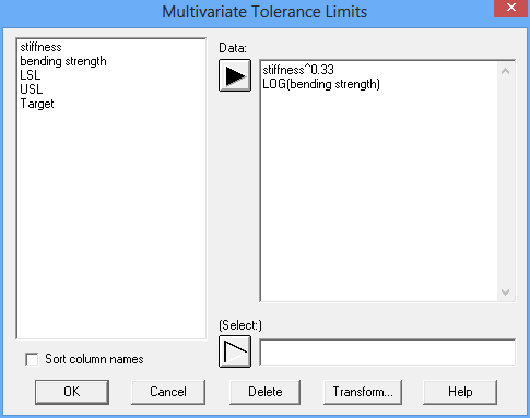
Step 3: Calculate the multivariate tolerance limits. In Statgraphics 18, select Describe – Numeric Data – Statistical Tolerance Limits – Multivariate Tolerance Limits. If a transformation has been selected, it should be indicated on the data input dialog box as shown below:

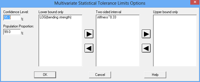
Use Analysis Options to specify C and P, and indicate the type of limits desired for each variable:

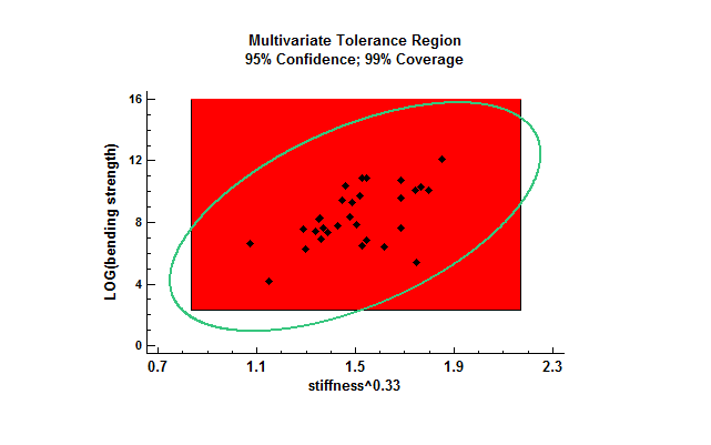
The multivariate tolerance limits will then be calculated and displayed in the transformed metric:

Further Information

The topics in this blog are described further in Chapter 7 of Polhemus (2018). I've also recorded a video on the topic: Multivariate Tolerance Regions (14:54).

References

Andrews, D.F., Gnanadesikan, R. and Warner, J.L. (1971), Transformations of Multivariate Data, Biometrics, 27, pp. 825-840.

Krishnamoorthy, K. and Mathew, T. (2009). Statistical Tolerance Regions: Theory, Applications, and Computation. John Wiley and Sons, Hoboken, N.J.

Polhemus, N.W. (2017). Process Capability Analysis: Estimating Quality. Boca Raton, FL: CRC Press.

Royston, J. P. (1983), Some Techniques for Assessing Multivariate Normality Based on the Shapiro-Wilk W, Applied Statistics, 32, pp. 121-133.