
Published under: new feature, statistical analysis, data analysis, Data analytics, Quality, Statgraphics, analytics software, design of experiments, screening designs, doe
The use of experimental design for process optimization is a well-established technique that encourages efficient use of experimental resources. It's one of those areas of statistical analysis where the ROI is relatively easy to quantify and can be extremely high. I still remember when Stu Hunter lectured to us in his course on DOE when I was an undergraduate engineering major. He began each lecture with a story about how he'd used what we were about to learn to help some company improve their processes. He had a unique knack for bringing real life into the classroom and encouraged many of us to pursue careers in statistics.
We spent a lot of time in that class talking about screening designs. Screening designs are experiments that involve simultaneously changing the levels of many input factors, with the goal of identifying those "vital few" factors which have the greatest impact on the response variables. We talked a lot about 2-level factorial and fractional factorial designs. We even learned how to use Yates' Algorithm to calculate effects (this was when handheld calculators were just appearing). Stu taught us about interactions, confounding, half-normal plots, and various other analysis techniques that could help identify the important factors. We also learned how to augment the original experiment by adding additional runs to enable us to fit a real response surface model in whatever factors turned out to be important.
In recent years, a class of experimental designs called "Definitive Screening Designs" have been developed that enable experimenters to fit a response surface model without doing additional runs. The initial set of runs has enough levels of each factor so that once insignificant factors have been eliminated, a second-order model with quadratic effects can be estimated in the remaining factors. Comparable in size to factorial experiments, they are a good alternative when curvature in the response variable is expected and the experimenter wants to avoid doing a second set of experimental runs. Statgraphics 18 includes definitive screening designs in its design catalog. Their construction and application is described in this blog.
Creating a DSD
As an example, let's suppose that we wanted to construct a screening experiment involving 5 factors. The example, which involves a chemical reaction, is discussed in Chapter 12 of the well-known book by Box, Hunter and Hunter (2005). The factors that will be varied are:
X1: feed rate
X2: amount of catalyst
X3: agitation rate
X4: temperature
X5: concentration
There is one response variable:
Y: percent reacted
In Box, Hunter and Hunter, they proceed by constructing a 16-run 25-1 fractional factorial design. Each factor is run 8 times at a low level and 8 times at a high level. The design is resolution V, meaning that there is no confounding amongst the main effects and the two-factor interactions. However, since there are only 2 levels of each factor, it is impossible to estimate quadratic effects of the factors.
As we shall see, a definitive screening design exists in 13 runs that provides an alternative to the fractional factorial design. We'll also discuss the strengths and weaknesses of the 2 design choices.
Step 1: Define response variables
To construct a definitive screening design using Statgraphics 18, we'll start with an empty datasheet and select DOE - Experimental Design Wizard from the main menu. Pressing Step 1: Define responses on the wizard toolbar, a single response variable will be defined:
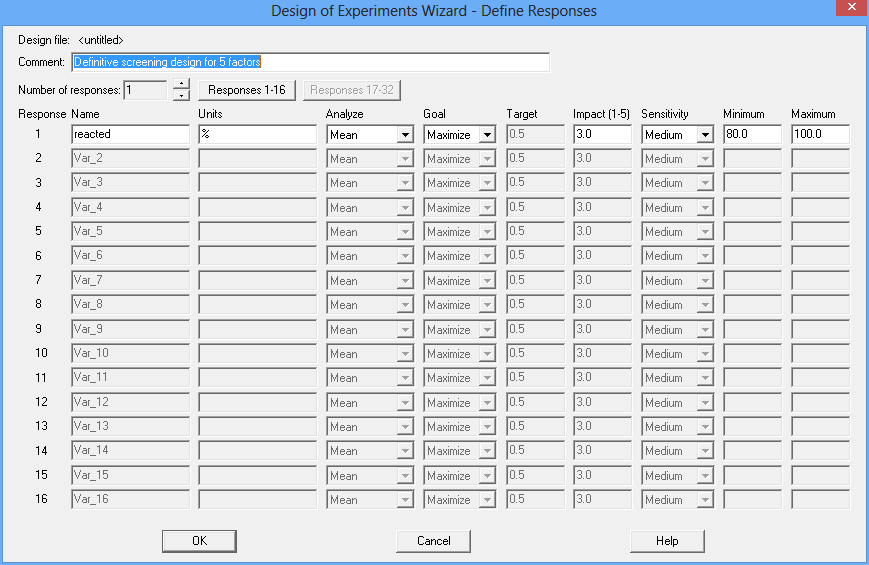
The goal of the experiment is to find a combination of the 5 factors that maximizes the percent reacted.
Step 2: Define experimental factors
After pressing Step 2: Define experimental factors on the wizard toolbar, 5 factors will be entered:
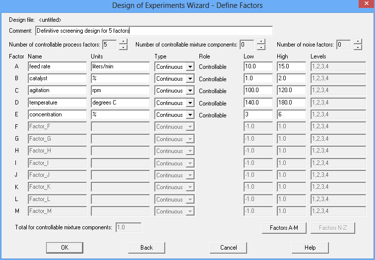
In this example, all 5 factors are continuous and may be run anywhere over the interval defined by the low and high values. Definitive screening designs, like 2-level factorial designs, may also include categorical factors provided they have only 2 levels.
Step 3: Select design
The third button on the DOE Wizard's toolbar is labeled Select design. To create a DSD, Screening is selected on the first dialog box:
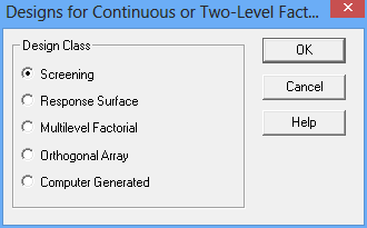
A second dialog box will then display a list of screening designs for 5 factors:
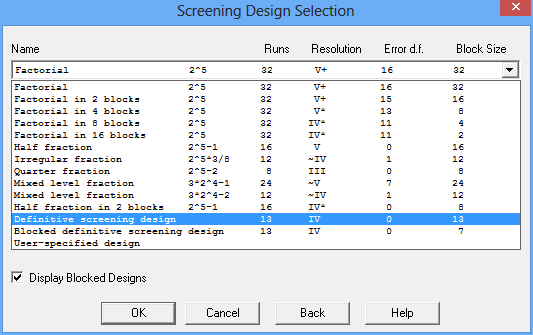
The list ranges from a full 2-level factorial design consisting of all 32 combinations of the low and high levels of the 5 factors to a quarter fraction in 8 runs. As noted earlier, the 25-1 half fraction is very popular since it is resolution V and therefore does not confound any of the main effects or 2-factor interactions. Since it is a fully saturated design leaving 0 degrees of freedom to estimate the experimental error, several additional runs are usually added at a central value of all the factors.
Near the bottom of the list are 2 definitive screening designs: one consisting of a single block of 13 runs, and the other consisting of 2 blocks with 7 runs in one block and 6 runs in the other. For designs containing m continuous factors run in a single block, the total number of runs in a DSD is
n = 2m’ + 1
where
m’ = m + k.
If m is even, k = 0, while if m is odd, k = 1. For designs run in B blocks where B > 1, the total number of runs is
n = 2m’ + B – k
The designs are constructed using conference matrices as described by Xiao, Lin and Bai (2012). For 5 continuous factors, the design is shown below:
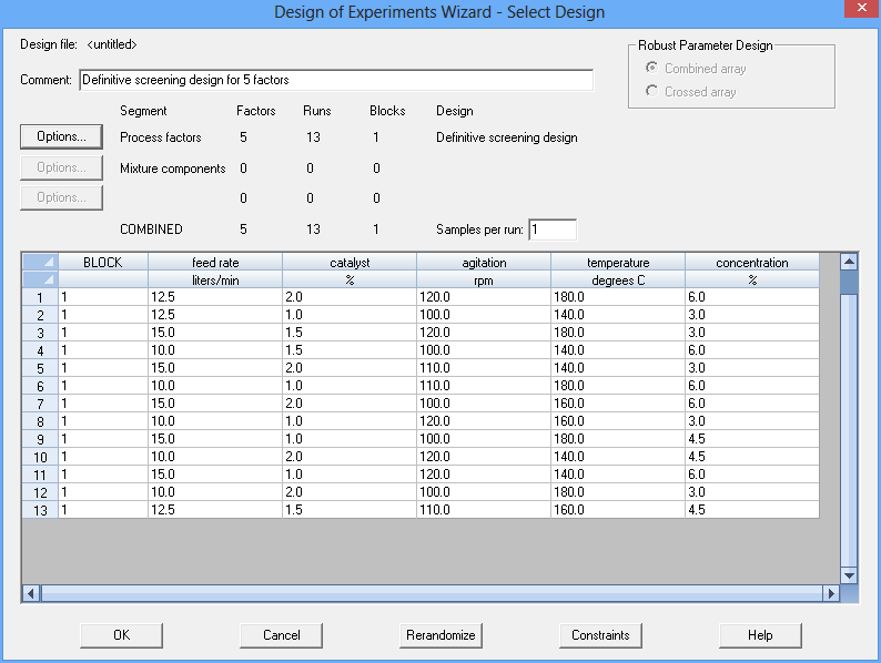
Notice that each factor is run 5 times at its low level, 5 times at its high level, and 3 times at a value halfway between the low and the high. Note also that the 3 central values for each factor are run once at the low level of every other factor, once at the high level of every other factor, and once at the central level of each factor. Since this design also has 0 degrees of freedom for estimating the experimental error, additional replicates of the centerpoint (run #13) would often be added to the design.
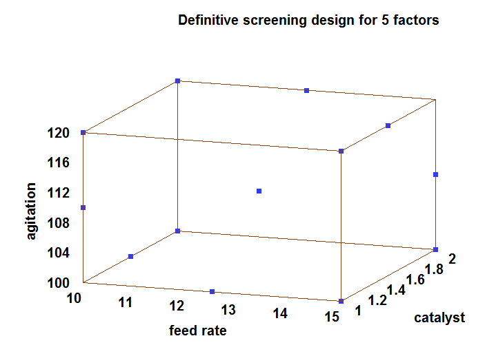
A projection of the design into the space of the first 3 factors is shown below:
Step 4: Specify model
Once the design has been created, the properties of the design may be studied. For 5 factors, the full second order model takes the following form:

There is a constant term, 5 main effects, 10 2-factor interactions, and 5 quadratic terms. Obviously, 13 runs is not sufficient to estimate this entire model, so only a subset may be fit.
In general, a definitive screening design has the following properties:
- Main effects are uncorrelated with each other, with the quadratic effects, or with the 2-factor interactions.
- Quadratic effects are uncorrelated with the main effects but have small correlations with each other. They are also correlated with the 2-factor interactions.
- 2-factor interactions are correlated with each other.
Suppose that initially, the experimenter is interested in screening all main effects and 2-factor interactions. In such cases, the 2-factor interaction model would be selected:
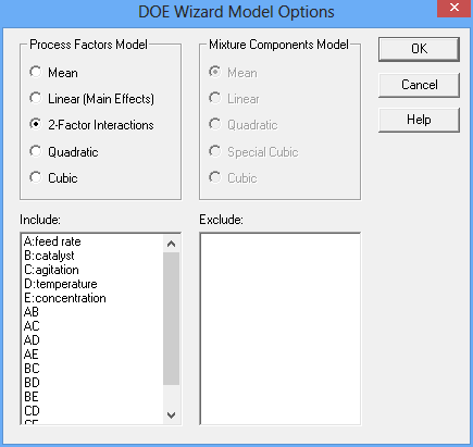
If we try to fit a model with all 5 main effects and 10 2-factor interactions, we'll quickly see that the DSD cannot estimate them all. For one thing, there are not enough runs. For another, certain 2-factor interactions are linear combinations of other interactions. The best that can be done is to estimate the 5 main effects and 5 of the 2-factor interactions:
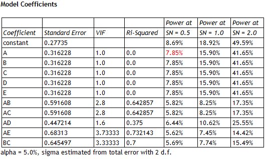
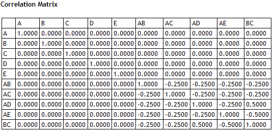
The selection of interactions in the above table is arbitrary; many other combinations are possible. Notice that the variance inflation factors (VIF) for the main effects equal 1.0, since the main effects are orthogonal to all of the other effects. There is some variance inflation in the estimated 2-factor interactions, but it is not dramatic. In fact, none of the correlation coefficients between the estimated effects exceed 0.5 in absolute value:
On the other hand, there is serious aliasing between the 2-factor interactions that are included in the model and those that are not. The table below shows the alias matrix for the selected model:
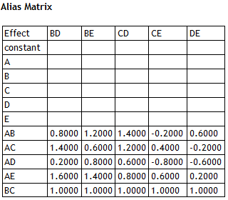
The alias matrix shows any potential bias in each estimated coefficient due to the effects that are not included in the model. For example:
![]()
As with other resolution IV designs, it may be possible to sense the presence of 2-factor interactions but they will be very difficult to identify.
On the other hand, if 3 factors appear to have large main effects, the full quadratic model may be fit in those factors:
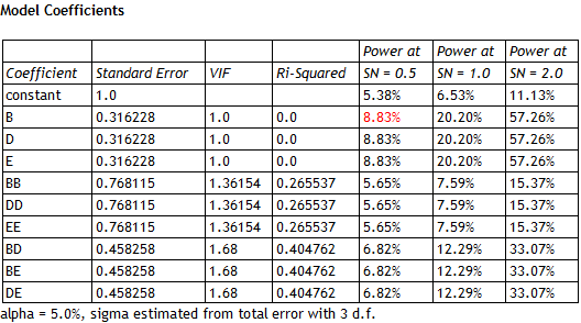
This illustrates the real attraction of the DSDs. Without running additional experiments, it is possible to get a reasonable estimate of the response surface in any 3 factors. Notice that the VIFs are relatively low, so the fitted model could well be used for process optimization. To fit such a model after running a 2-level fractional factorial design, additional experiments would need to be done, such as adding star points to create a central composite design.
Application
To examine how DSDs work in practice, let's suppose that the actual underlying model for % reacted in the chemical process described above is

% reacted equals 95 when catalyst = 2 (its high level in the design), temperature = 200 (greater than its high level), and concentration = 4.5 (midway between its low and high levels). The factors feed rate and agitation have no effect on the response. The data below show simulated values for each of the 13 runs in the DSD experiment, adding a random error to each observation generated from a normal distribution with m = 0 and s = 0.1:
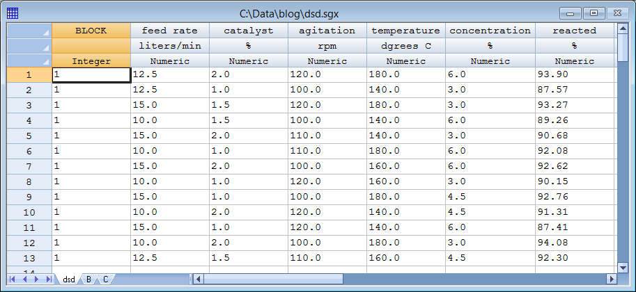
Suppose we start by fitting a model with all 5 main effects and 5 2-factor interactions. The standardized Pareto chart for such a model is shown below:
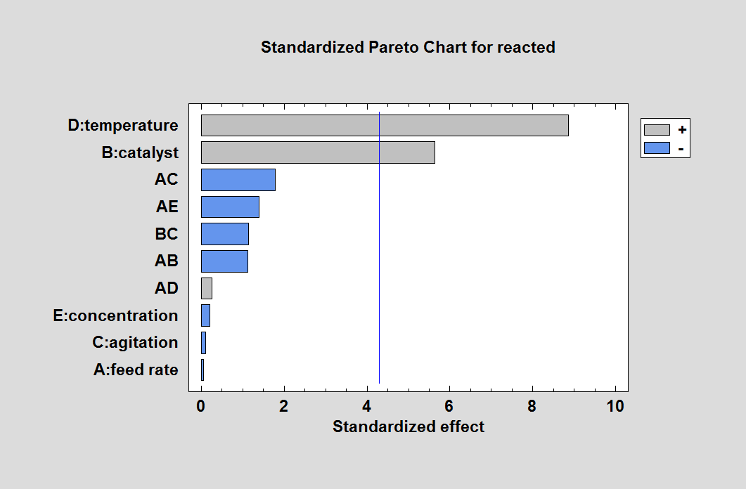
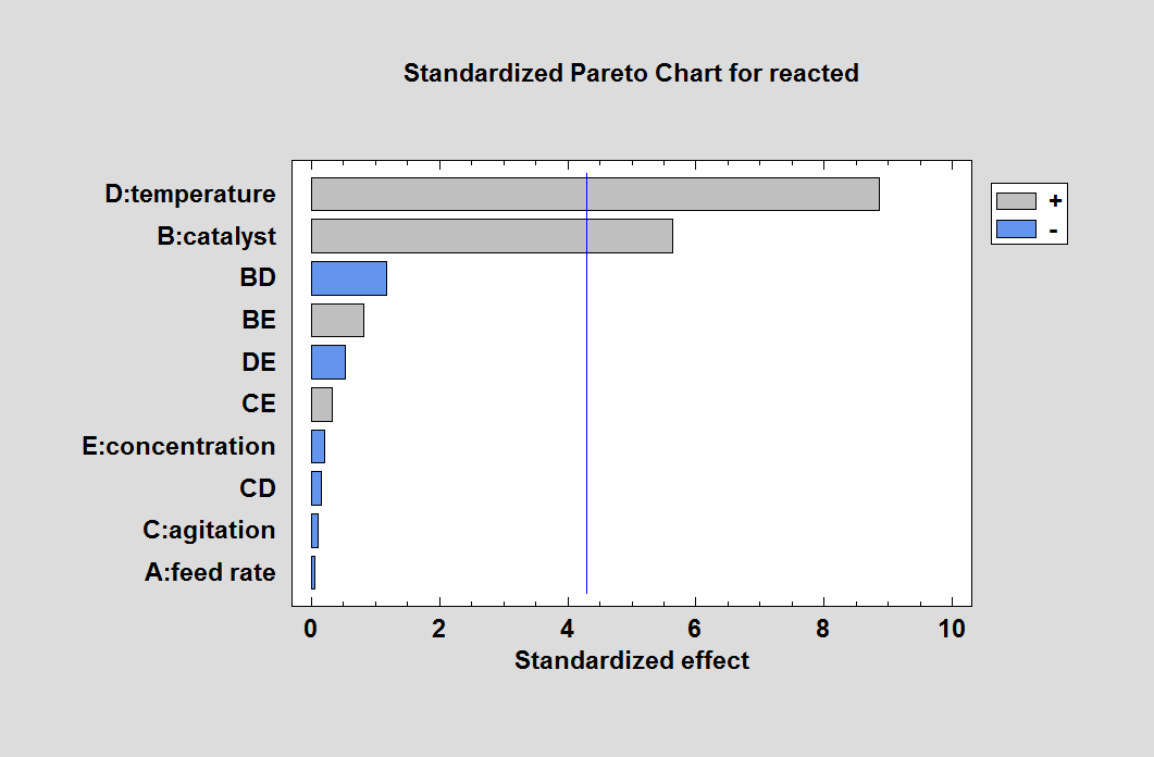
Since the fitted model contains 11 coefficients including the grand average, the residual mean squared error has only 2 degrees of freedom. Consequently, the t-value for each individual coefficient must be in excess of 4.3 to be statistically significant at the 5% significance level. Temperature and catalyst both exceed that value and are clearly identifiable. The estimated main effect of concentration (which peaks in the center of the experimental region) is very small. None of the 2-factor interactions are close to being statistically significant. Even if we happened to select a set of interactions containing BD (which is included in the model), the results are similar:
Another analysis possibility is to remove all 2-factor interactions but include all quadratic effects. This is something that could not be done with a fractional factorial design. For the sample data, the result is shown below:
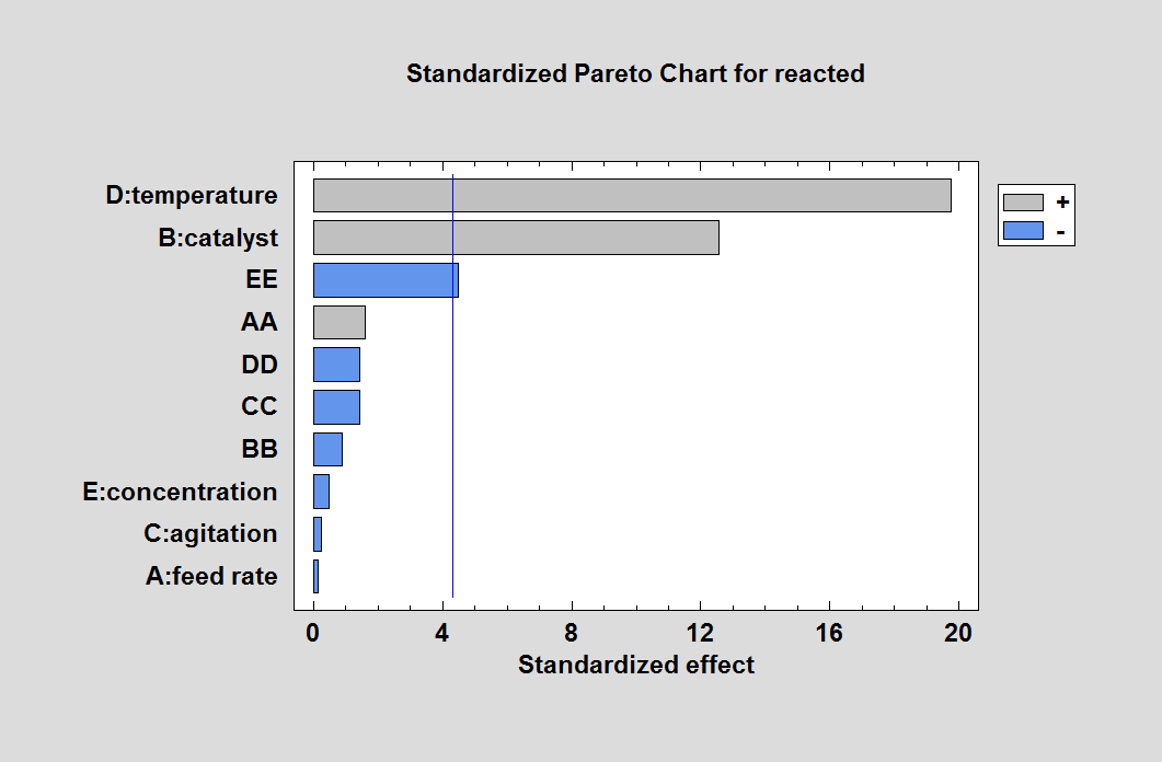
The importance of concentration is now evident through the term "EE", which represents its quadratic effect. At this point, we would have correctly identified the 3 active factors, although we haven't yet detected the interaction between temperature and catalyst.
Since our DSD is capable of fitting a full quadratic model in any 3 factors, another analysis strategy would be to fit full quadratic models for all combinations of 3 factors and compare the results. The table below shows the mean squared error and R-squared statistic for the 10 possible combinations:
| Factors | MSE | R-squared |
| A,B,C | 13.1553 | 32.82% |
| A,B,D | 0.0101 | 99.95% |
| A,B,E | 13.1497 | 32.85% |
| A,C,D | 5.3168 | 72.85% |
| A,C,E | 18.4565 | 5.75% |
| A,D,E | 5.3112 | 72.88% |
| B,C,D | 0.0087 | 99.96% |
| B,C,E | 13.1483 | 32.86% |
| B,D,E | 0.0040 | 99.98% |
| C,D,E | 5.3098 | 72.88% |
The combination with the lowest MSE and highest R-squared is "B,D,E", which does contain the 3 factors that were present in the model from which the data were generated. Note that 2 other combinations are also quite good: "A,B,D" and "B,C,D". These combinations substitute either factor A or factor C for the correct factor E. Looking at the alias matrix for the model involving factors A, B and D, you can see that the missing quadratic effect EE is aliased with 4 of the terms contained in that model:
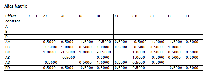
However, in the end, the experimenter would probably have correctly identified factors B, D and E as the active factors. The Pareto chart for the full quadratic model in those factors is shown below:
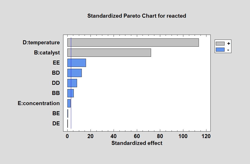
The Pareto chart correctly identifies the active terms in the model from which the data were generated.
Optimization
Having selected a model, Statgraphics 18 may then be asked to optimize the response. The results are shown in the following table:
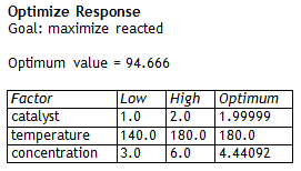
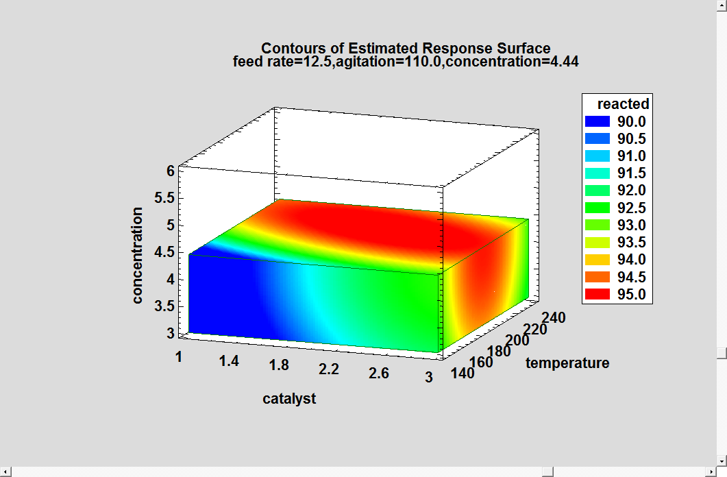
The optimum values of catalyst and temperature are spot on, which the optimum value of concentration is close to the true value of 4.5. You can tell by the 3-dimensional contour plot of reacted that there is a large region around the final solution that results in almost identical results:
A slightly different view is provided by the 3D mesh plot:
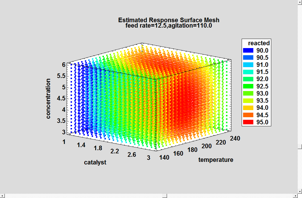
A response close to 95% is obtainable throughout the entire range of concentration. You can also see the effect of the interaction between catalyst and temperature, with the optimum value of one depending on the value of the other. .
Conclusion
The definitive screening designs provide a way to both identify the most important factors and optimize the response variable using a single set of experimental runs. As such, they are an economical solution for experimenters whose final goal is process optimization.
References
Box, G. E. P., Hunter, W. G. and Hunter, J. S. (2005). Statistics for Experimenters: An Introduction to Design, Data Analysis, and Model Building, 2nd edition. New York: John Wiley and Sons.
Jones, B. and Nachtsheim, C.J. (2011) “A Class of Three-Level Designs for Definitive Screening in the Presence of Second-Order Effects”, Journal of Quality Technology 43(1), pp. 1-15.
Jones, B. and Nachtsheim, C.J. (2013) “Definitive Screening Designs with Added Two-Level Categorical Factors”, Journal of Quality Technology 45(2), pp. 121-129.
Jones, B. and Nachtsheim, C.J. (2016) “Blocking Schemes for Definitive Screening Designs”, Technometrics 58(1), pp. 74-83.
Xiao, L., Lin, D.K.J. and Bai, F. (2012) “Constructing Definitive Screening Using Conference Matrices”, Journal of Quality Technology 44(1), pp. 1-7.

 By:
By: 


