The simplest statistical relationship between a dependent variable Y and one or more independent or predictor variables X₁, X₂, ... is 

Y = B₀ + B₁X₁ + B₂X₂ + ... + e

where e represents a random deviation from the mean relationship represented by the rest of the model. With a single predictor, the model is a straight line. With more than one predictor, the model is a plane or hyperplane. While such models are adequate for representing many relationships (at least over a limited range of the predictors), there are many cases when a more complicated model is required.

In Statgraphics, there are several procedures for fitting nonlinear models. The models that may be fit include:

1. Transformable nonlinear models: models involving a single predictor variable in which transforming Y, X or both results in a linear relationship between the transformed variables.

2. Polynomial models: models involving one or more predictor variables which include higher-order terms such as B_1,1X₁² or B_1,2X₁X₂.

3. Models that are nonlinear in the parameters: models in which the partial derivatives of Y with respect to the predictor variables involve the unknown parameters.

While the first 2 types of models may be fit using linear least squares techniques, the third requires a numerical search procedure.

In this blog, I will show examples of the 3 types of models and give some advice on fitting them using Statgraphics.

Fitting Transformable Nonlinear Models

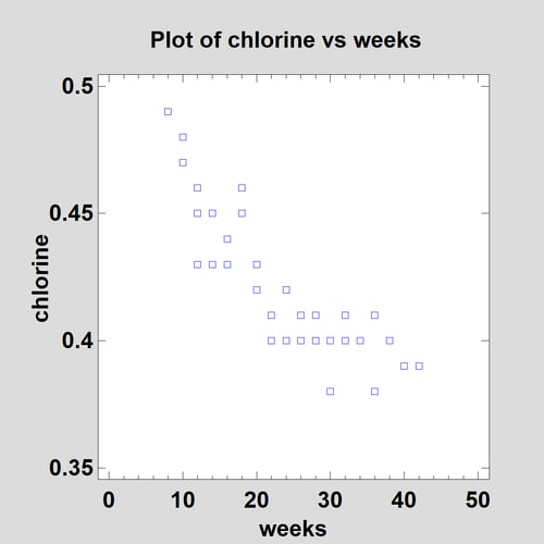
In their classic book on regression analysis titled Applied Regression Analysis, Draper and Smith show a data set containing 44 samples of a product in which the active ingredient was chlorine. Researchers wanted to model the loss of chlorine as a function of the number of weeks since the sample was produced. As is evident in the scatterplot below, chlorine decays with time:

In order to get a quick feel for the shape of the relationship, a robust Lowess smooth may be added to the plot:

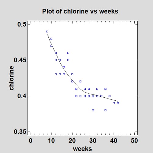
Lowess stands for "Locally Weighted Scatterplot Smoothing" and was developed by Bill Cleveland. It smooths the scatterplot by fitting a linear regression at many points along the X axis, weighting observations according to their distance from that point. The procedure is then applied a second time after down-weighting observations that were far removed from the result of the first smooth. It may be seen that there is significant nonlinearity in the relationship between chlorine and weeks.

The Simple Regression procedure in Statgraphics gives a choice of many nonlinear functions that may be fit to this data:

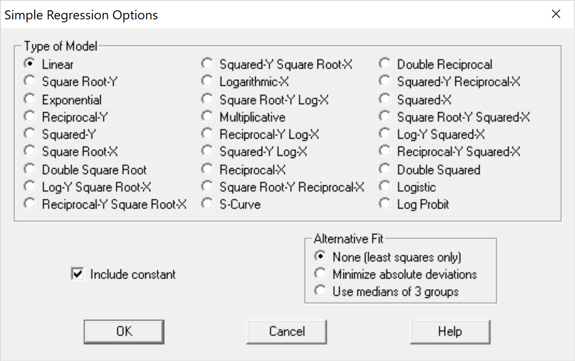
Each function has a form such that after transforming Y, X or both appropriately, the model will be linear in the parameters. For example, the multiplicative model takes the form

Y = a X^B

which may be linearized by taking logs of both variables:

ln(Y) = ln(a) + B ln(X)

The one caveat in such an approach is that the error term e is assumed to be additive after the model has been linearized.

To help select a good nonlinear model, Statgraphics will fit all of the models and sort them in decreasing order of R-squared:

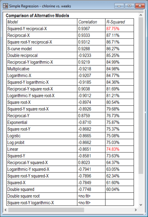
The R-squared displayed is calculated in the transformed metric, so it represents how well a straight line fits the transformed data. Models near the top of the list are worth considering as alternatives to a linear model. The Squared-Y reciprocal-X model has the form

Y² = B₀ + B₁/X

while the Reciprocal-X model is

Y = B₀ + B₁/X

When I'm building empirical models and the results of 2 models are very similar, I usually pick the simpler of the two. Fitting a Reciprocal-X model to this data gives the following curve:

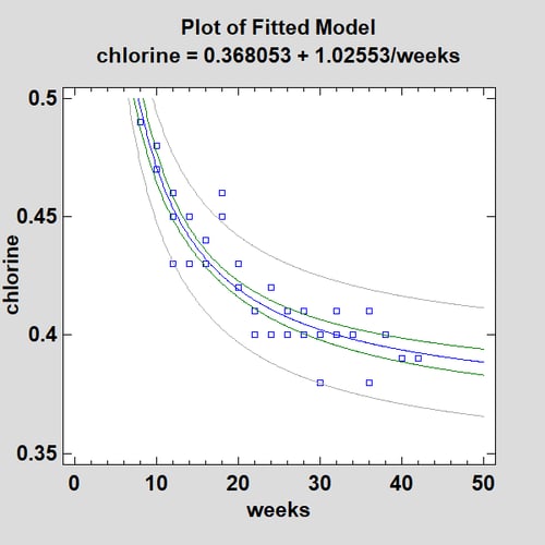
In addition to fitting the general relationship well, this model has the pleasing property of reaching an asymptotic value of 0.368053 when weeks becomes very large.

Draper and Smith noted the 2 apparent outliers at weeks = 18. The Statgraphics Table of Unusual Residuals shows that the Studentized residuals for those observations both exceed 2.4:

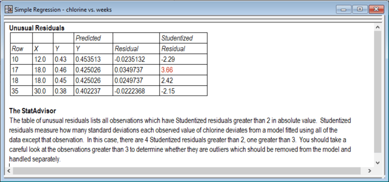
In particular, row #17 is 3.66 standard deviations from its predicted value. However, since they could find no assignable cause that would justify removing those points, Draper and Smith left them in the dataset.

Fitting Polynomial Models

Rather than transforming Y and/or X, we might try fitting a polynomial to the data instead. For example, a second-order polynomial would take the form

Y = B₀ + B₁X + B₂X²

while a third-order polynomial would take the form

Y = B₀ + B₁X + B₂X² + B₃X³

Since polynomials are able to approximate the shape of many curves, they might give a good fit.

The Polynomial Regression procedure in Statgraphics fits polynomial models involving a single Y and a single X. The Analysis Options dialog box lets the user specify both the order of the polynomial and a shift parameter D:

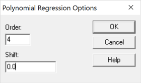
A fourth-order model with a non-zero shift parameter takes the form

Y = B₀ + B₁(X-D) + B₂(X-D)² + B₃(X-D)³ + B₄(X-D)⁴

By specifying a non-zero value for D, the origin of the polynomial is shifted to a different value of X which can prevent the powers from becoming so large that they overflow the variables created to hold them when performing calculations. Since the maximum value of X is not large in our sample data, the shift parameter may be set equal to 0.

For the chlorine, a fourth-order polynomial fits the data quite well:

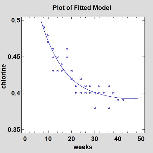
In fact, if we overlay the Reciprocal-X model and the fourth-order polynomial in the StatGallery, the predictions are very similar throughout the range of the data:

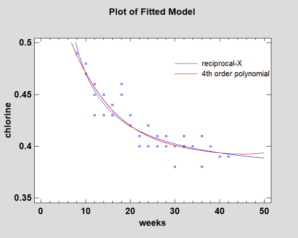
However, beyond the range of the data the polynomial will behave erratically. While the polynomial is suitable if we are only doing interpolation, the Reciprocal-X model would be preferred if extrapolation is required.

From a statistical point of view, the 4th order polynomial may be more complicated than is required. Statgraphics creates a table that may be used to help determine what order of polynomial is needed to sufficiently capture the relationship between Y and X. Called the Conditional Sums of Squares table, it tests the statistical significance of each term in the polynomial when it is added to a polynomial of one degree less:

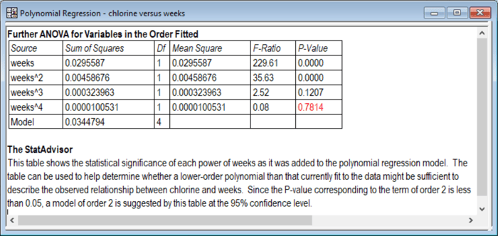
For example, when X² is added to a linear model, the P-Value for B_² equals 0.0000, implying that it significantly improves the fit. When X³ is added to a second-order model, the P-Value for B_³ equals 0.1207, implying that it does not significantly improve the fit at the 10% significance level. In this case, the P-Values suggest that a second-order polynomial would be sufficient. However, a plot of the fitted model might give one pause:

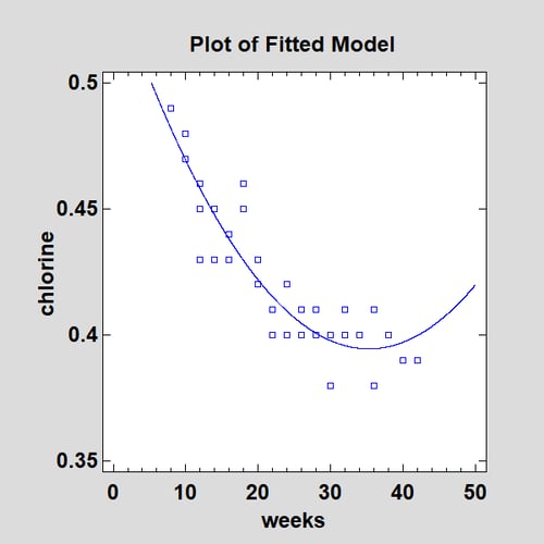
Even if only using the model for interpolation, the curvature in the interval between 30 and 40 weeks is disconcerting.

Fitting Models which are Nonlinear in the Parameters

All of the models fit above are "linear statistical models" in the sense that (at least after transforming Y and/or X), the models may be estimated using linear least squares. A linear statistical model is one in which the partial derivatives of the function with respect to each parameter do not contain any of the unknown parameters. An example of a nonlinear model that cannot be linearized by transforming the variables is

Y = a + (0.49-a)e^-B(X-8)

Yet such a model might be quite reasonable for this data since it implies that the amount of chlorine in each sample equals 0.49 at 8 weeks and then decays to an unknown asymptotic level a at an unknown rate B. This is in fact the model suggested by the researchers from whom Draper and Smith obtained the sample data.

Finding estimates of a and B that minimize the residual sum of squares for the above model requires a numerical search. The Nonlinear Regression procedure in Statgraphics lets users fit such models by entering them on the following data input dialog box:

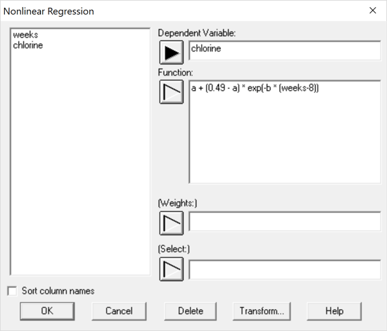
When evaluating a function, any terms that don't correspond to columns in the active datasheets are considered to be unknown parameters. The user must also enter starting values for the unknown parameters to determine the location at which the numerical search begins:

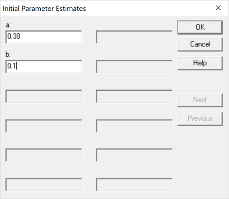
Based on the models fit earlier, a good starting estimate for the asymptotic value a is 0.38. Less is known about the rate parameter B. In such cases, it often suffices to set the starting value to either 0.1 or -0.1. It is important that the sign be correct, however, since the search algorithms sometimes have trouble if they need to cross 0.

The Analysis Options dialog box lets the user control the search procedure:

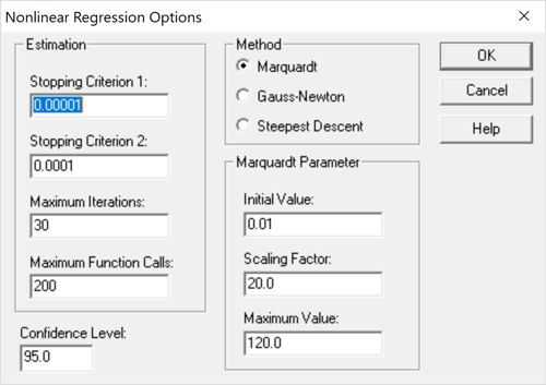
Normally, the default settings here are adequate to find a good model. Of particular interest are the stopping criterion and the search method. By default, the search will stop and be declared successful if either the relative change in the residual sum of squares between 2 consecutive iterations is less than Stopping Criterion 1 or the relative change in all parameter estimates is less than Stopping Criterion 2. If the search does not succeed, you can try increasing the maximum number of iterations and function calls or switching from the Marquardt method to one of the other choices. More often, selecting a better set of starting values for the parameters will lead to a successful fit.

The resulting fit is shown below:

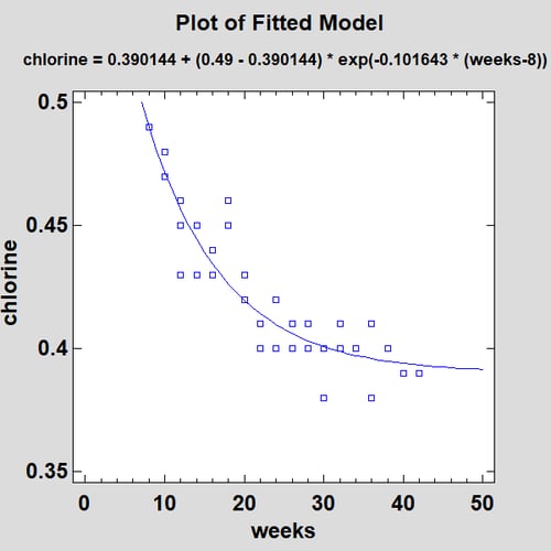
The fitted model is very similar to the Reciprocal-X model.

Example 2: Nonlinear Model with 2 Predictors

There are times when you'd like to fit a model that is linearizable such as 

Y = exp(B₀ + B₁X₁ + B₂X₂ + B₃X₁X₂)

but where the errors are additive in the original metric rather than the transformed metric. For example, consider the following data from an experiment where 38 observations have been taken from a process in which yield is a function of time and temperature:

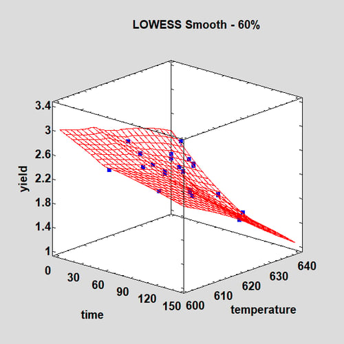
The data are shown with a two-dimensional LOWESS smooth. The relationship is clearly nonlinear.

To fit the nonlinear function desired while retaining additive errors, we would proceed as follows:

1. Fit the function LOG(Y) = B₀ + B₁X₁ + B₂X₂ + B₃X₁X₂ using the Multiple Regression procedure. This assumes multiplicative errors in the original metric of yield.

2. Fit the function Y = exp(B₀ + B₁X₁ + B₂X₂ + B₃X₁X₂) using the Nonlinear Regression procedure, using the estimated coefficients from Step #1 as the starting values for the unknown parameters. This assumes additive errors in the original metric of yield.

The resulting fit is shown below:

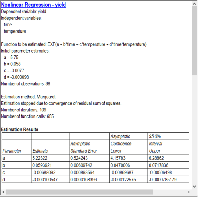
Notice that the number of iterations needed to be increased to 120 in order for the algorithm to meet the stopping criteria.

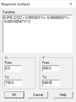
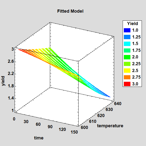
We can plot the final model using the Statgraphics Surface and Contour Plots procedure:

The plot below displays the function using a ribbon plot:

Conclusion

Nonlinear models often capture the relationships in a set of data better than linear models. In Statgraphics, several procedures are provided to fit such models and display the results. It should be remembered that the goal of building empirical models is not necessarily to provide a complete explanation of the observed phenomena. Rather it is to create models that give useful predictions within the range of the observed data. Using a sufficiently detailed model to capture the underlying relationship is important, but it should not be so complex that it captures random variations. Often, remembering to Keep It Simple Statistically (KISS) leads to the most successful results.

References

Cleveland, William S. (1979), "Robust Locally Weighted Regression and Smoothing Scatterplots", Journal of the American Statistical Association 74 (368), 829-836.

Draper, N.R., and Smith, H. (1998), Applied Regression Analysis, third edition, John Wiley and Sons.

Statgraphics Technologies, Inc. (2018) Statgraphics, www.statgraphics.com