One of the most heavily used sections of Statgraphics is that containing procedures for regression analysis. Each of the procedures is designed to predict the value of a dependent variable Y based on the values of one or more factors. Depending on the type of data in Y, users may select:

1. For continuous Y, procedures such as General Linear Models, Nonlinear Regression, Orthogonal Regression, and several others.

2. For binary Y or proportions, procedures such as Logistic Regression and Probit Analysis.

3. For count data, procedures such as Poisson Regression, Negative Binomial Regression, and Zero-Inflated Count Regression.

4. For life data or times to failure, procedures such as Cox Proportional Hazards or Life Data Regression.

The newest release of Statgraphics (V19.5) contains 2 new procedures for fitting regression models when Y is categorical:

5. Ordinal Regression when Y consists of ordered categories.

6. Multinomial Logistic Regression when Y consists of unordered categories or when the proportional odds assumption of ordinal regression does not hold.

ORDINAL REGRESSION

As an example, the UCI Machine Learning Repository contains a dataset in which 913 faculty members at 2 Spanish universities were surveyed about their perceptions of the usefulness of Wikipedia. They were asked a series of questions to which they responded using the following Likert scale:

1 = strongly disagree

2 = disagree

3 = neutral

4 = agree

5 = strongly agree

This is a case where the response is ordinal. Each faculty member was also classified in several ways:

AGE: numeric
GENDER: male or female
DOMAIN: 1=Arts & Humanities; 2=Sciences; 3=Health Sciences; 4=Engineering & Architecture; 5=Law & Politics
PhD: 0=No; 1=Yes
YEARSEXP (years of university teaching experience): numeric
UNIVERSITY: 1=UOC; 2=UPF

The goal here is to develop a predictive model for a faculty member's response based on these factors.

In this blog, we will concentrate on the response to the following statement, labeled Qu1: "Articles in Wikipedia are reliable." We will start with a very simple model involving only one predictive factor: AGE. Letting Y take k  values between 1 and 5, we'll first transform the probability that Y ≤ j using the logit transformation

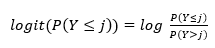
The logit transformation is the logarithm of the odds that Y is less than or equal to j. In an ordinal regression model, the logit transformation is related to the predictor variables according to

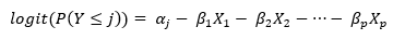
There is a separate intercept α_j for each of first k-1 unique values of Y and a common parameter for each of the p values of X. The intercepts each correspond to a breakpoint between the levels of the ordinal variable Y, in this case between strongly disagree vs disagree,  between disagree vs neutral, and so on. There is a single β parameter for each quantitative predictor and (m-1) β parameters for categorical factors that have m levels. Note that each β coefficient is preceded by a negative sign. This is intentional so that when β is positive, increasing the value of X causes a decrease in the odds that Y ≤ j,  which corresponds to a more favorable response.

Examining the model, it should be noted that the effect of the predictors does not depend on j. The logit curves as a function of X simply shift upward at each breakpoint. This is called the proportional odds or parallel regression assumption. If this assumption is not tenable, then we would need to do a full multinomial fit that does not rely on the special structure of ordinal data.

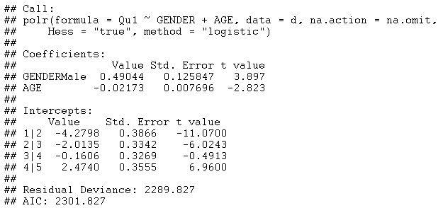
To analyze this data in Statgraphics, we will begin with a model involving only AGE. Statgraphics calls the POLR function in R to do the calculations, which returns the following tables:

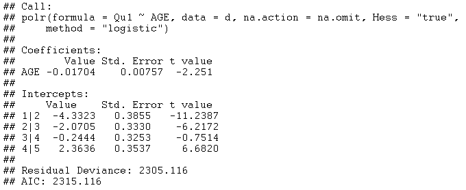
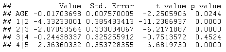
The small P-Value for AGE indicates that the effect of age on the response is statistically significant at the 5% significance level. The negative coefficient indicates that AGE has a positive effect on the odds of being less than or equal to j (recall that the model contains negative signs before each coefficient). This indicates that older faculty members have a less favorable attitude toward the reliability of Wikipedia.

The fitted model can be examined by decoding the fitted model and plotting the probabilities that Y = j for each value of j:

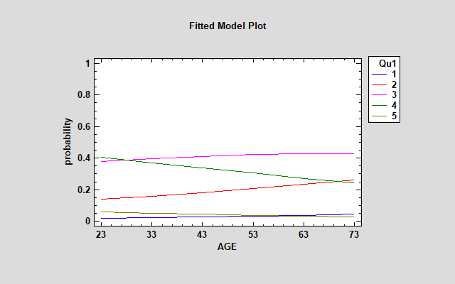
The effect of AGE is particularly noticeable for j = 2 and 4. Older faculty members are much more likely to "disagree" while younger members are more likely to "agree".

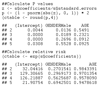
To make the model more interesting, we will now introduce GENDER as a categorical factor. As seen in the following output, GENDER is also statistically significant at the 5% significance level:

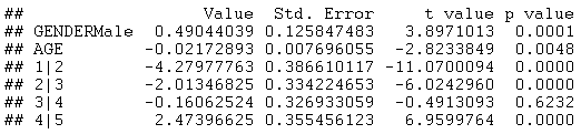
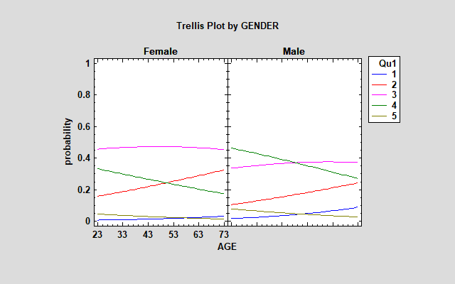
The positive value on GENDERMale indicates that when GENDER = Male, the value of the logit function goes down by 0.49. This equates to a more favorable response. The difference between males and females is quite noticeable when plotting probabilities in a trellis plot:

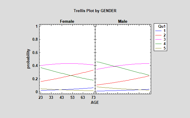
Females are more likely to respond with "disagree" or "strongly disagree" and males with "agree" or "strongly agree".

Different models can be compared by looking at the Akaike Information Criterion (AIC). AIC is an estimate of prediction error that takes into account the number of estimated parameters. Since the second model has a lower value of AIC, it is preferable to the first model.

There are also various options that can be set when fitting an ordinal regression model, as seen on the Analysis Options dialog box:

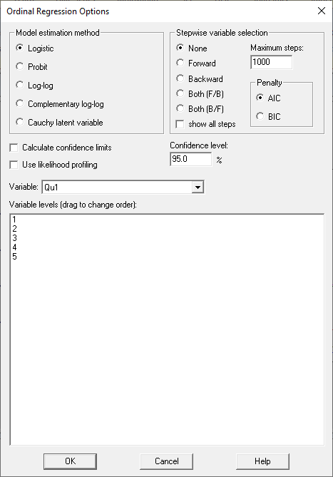
Instead of using the logistic transformation, other link functions such as the Probit may be used. It has been suggested that:

1. Logistic be used when all categories have similar probabilities.

2. The log-log function be used when lower categories are dominating.

3. The complementary log-log function be used when higher categories are dominating.

4. The Cauchy latent variable transformation be used when there are extreme values.

In addition, stepwise variable selection may be conducted to select a subset of possible predictor variables. Adding DOMAIN, PhD, YEARSEXP and UNIVERSITY to the model and selecting Forward stepwise variable selection results in the following model:

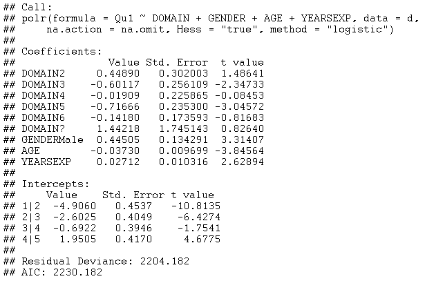
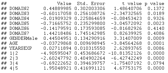
All variables except PhD and UNIVERSITY were selected by the stepwise variable selection procedure. The large negative coefficients on DOMAIN3 and DOMAIN5 are particularly interesting. They imply that faculty members in those domains are more likely than others to have an unfavorable opinion about the reliability of Wikipedia articles.

MULTINOMIAL REGRESSION

If the k categories of the dependent variable Y have no natural order, then a multinomial regression must be done instead of an ordinal regression. This involves fitting a model of the form

This model describes the effects of the predictive factors on the ratio of the probability for category j to the probability for category 1. There is a full set of β's for each category except category 1. Note that this allows the effect of the factors to be different for each category.

Statgraphics fits such models by calling the multinom function in R. For the model involving AGE and GENDER, the output is shown below:

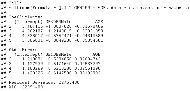
The model has twice as many parameters as the ordinal regression model (12 versus 6). The AIC is slightly smaller (2299.488 versus 2301.827). Notice that the estimated coefficients for each GENDERMale vary considerably amongst the responses 2 through 5.

Examining the trellis plot for this model, you will notice the same basic pattern in the estimated probabilities as with the ordinal regression model.

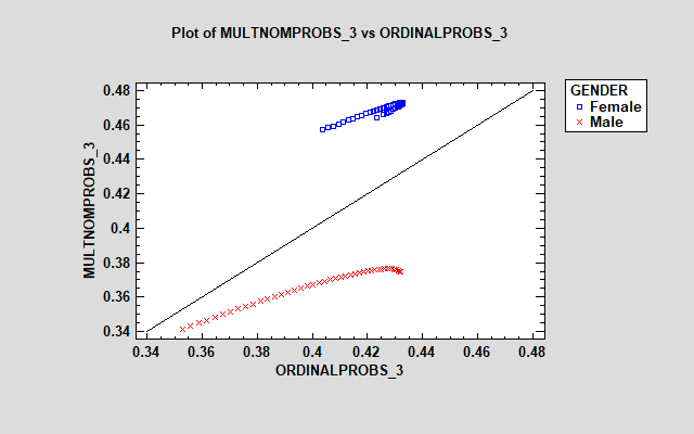
However, the blue line for older males is quite a bit higher than in the ordinal model. An interesting way to compare the ordinal and multinomial regression results is to save the estimated probabilities for each faculty member from both models and construct plots such as that shown below:

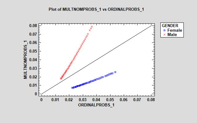
The plot shows the estimated probability that each individual will respond "strongly disagree" based on their age and gender. The multinomial regression model predicts a considerably higher probability for males, while the ordinal model predicts a higher probability for females. The effect of age, shown by the range of the points, is also more pronounced for males in the multinomial model. Similar plots could be generated for each of the other responses. 

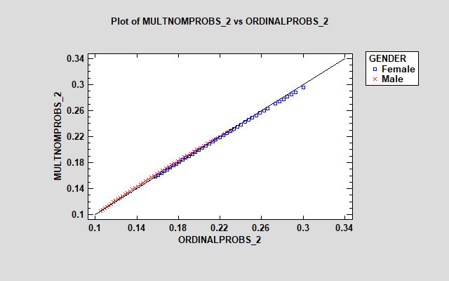
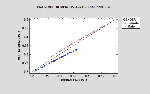
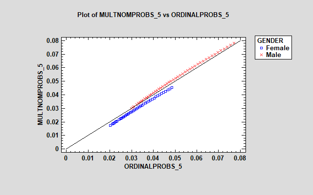
The models are reasonably similar for responses 2, 4 and 5. However, there is a large discrepancy between the models for the "neutral" response (3), with the multinomial model showing much larger estimated probabilities for females. The additional parameters in the multinomial model let it treat the effect of the factors on each response differently.

To determine whether the additional parameters for the multinomial model can be justified statistically, an approximate likelihood ratio test can be calculated from the residual deviances:

G = 2289.827 - 2275.488 = 14.339

which may be compared to a chi-square distribution with 12-6 = 6 degrees of freedom. The P-value for this statistic is approximately 0.026, leading to the conclusion that the multinomial model is preferable at the 5% significance level.

REFERENCES

Data source: Dua, D. and Graff, C. (2019). UCI Machine Learning Repository [http://archive.ics.uci.edu/ml]. Irvine, CA: University of California, School of Information and Computer Science. https://archive.ics.uci.edu/ml/datasets/wiki4he

Citation: Meseguer, A., Aibar, E., Lladós, J., Minguillón, J., Lerga, M. (2015). Factors that influence the teaching use of Wikipedia in Higher Education. JASIST, Journal of the Association for Information Science and Technology. ISSN: 2330-1635. doi: 10.1002/asi.23488.