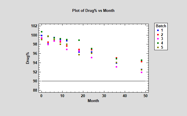
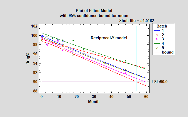
Determining the shelf life or retest period for a product or substance requires modeling the degradation of that product over time. In the case of drug substances, it is common to take samples from multiple batches and determine when the confidence limit for the batch means falls below the specification limit. For example, the plot below shows data from 5 batches measured at intervals ranging from 0 to 48 months after production. The specification limit is set at 90% of the label-claimed active ingredient strength of the drug.

In modeling this data, 2 primary questions must be answered:

1. What type of mathematical function best describes the degradation of the drug over time? A linear relationship? A nonlinear  relationship? If nonlinear, is it exponential or some other form?

2. Are there significant differences between the batches? Is so, should we fit a separate function to each batch or treat batches as another random source of variability?

Fixed Batch Effects Model

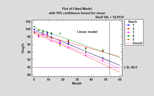
In looking at the FDA's Guidance for Industry, it appears that the most common approach is to collect data from a minimum of 3 batches, fit a separate linear relationship to each batch, and take the smallest shelf life determined for each batch. The plot below shows linear models fit to each batch, together with a lower confidence bound for the mean as a function of time. The confidence bound that is plotted connects the smallest lower 95% confidence bound amongst the 5 batches at each point in time. It results in an estimated shelf life of approximately 52.8 months.

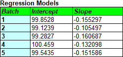
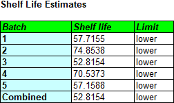
The tables below show the estimated intercepts and slopes for each model, together with the shelf life estimates.

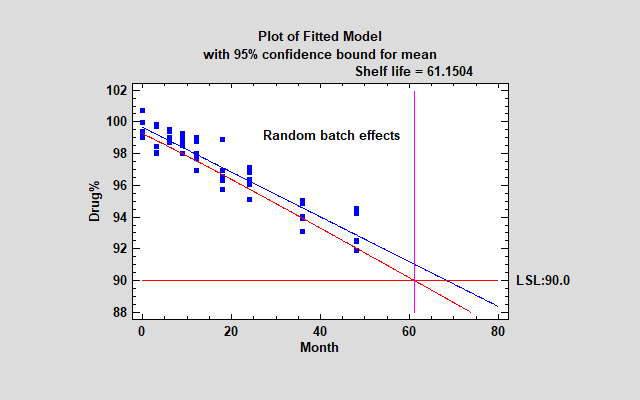
Fitting separate models to each batch and taking the most conservative result could easily result in a lower shelf life than fitting a single line to all of the data. For the current data, pooling all of the batches results in a shelf life estimate of 65.0 months. Pooling is only legitimate for the fixed effects model, however, if there are not significant differences between the models fit to the 5 batches. That can be tested by looking at the Analysis of Variance (ANOVA) table:

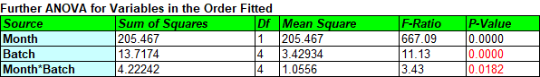
A small P-value for Month*Batch indicates that the slopes are significantly different while a small P-value for Batch indicates that the intercepts are significantly different. How small? According to the FDA guidelines, "Each of these tests should be conducted using a significance level of 0.25 to compensate for the expected low power of the design due to the relatively limited sample size in a formal stability study." Unless the P-values are greater than 0.25, the batches cannot be pooled. Note: Test the Month*Batch interaction first. If it is not significant, simplify the model and retest the Batch effects. Don't remove Batch if you keep Month*Batch.

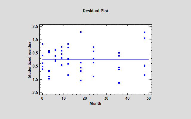
One other concern remains: use of the linear model. Whenever you are fitting regression models, it's a good idea to plot the residuals. Below you see a plot of the residuals from the fitted stability model versus time.

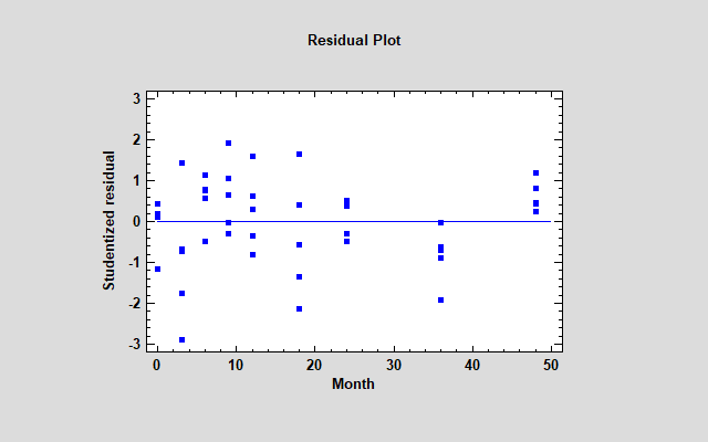
Actually, the vertical axis displays the Studentized residuals, which show how far each sample would be from the fitted model if the model was fit without that sample. One of the 3-month residuals equals -2.88, which is moderately large for only 50 residuals. More disturbing however is the fact that all 5 samples at 36 months are negative while all 5 samples at 48 months are positive. That's a suggestion that some curvature may be present.

To find out how much better a model we could fit to the data without overmodeling it, it's useful to try a number of transformable  nonlinear models. These are models which, after transforming Y or X or both, are linear for the transformed data. The Stability Studies procedure in Statgraphics 19 automatically tries up to 25 such models and lists the results in decreasing order of R-squared. (Note: Since Month contains values equal to 0, some of the models cannot be fit.)

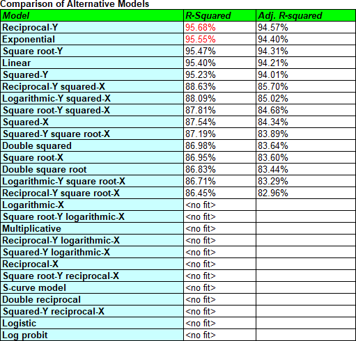
The Reciprocal-Y model has the highest R-squared value. In that model, 1/Y is a linear function of X. Looking at the fitted model, you'll see that it increased the shelf life estimate slightly but really didn't make much practical difference.

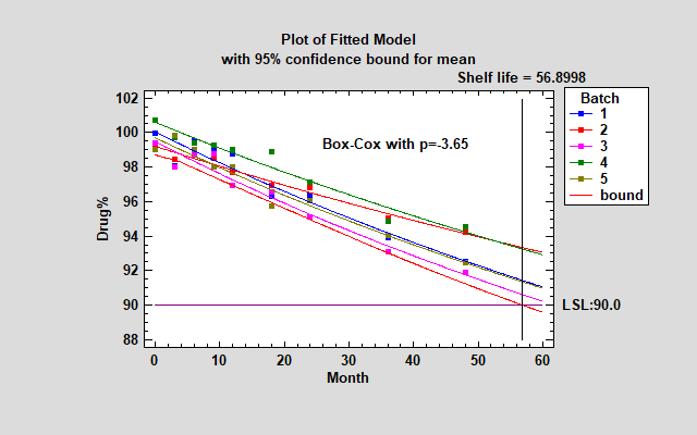
Another possible approach is to try a Box-Cox transformation. A Box-Cox transformation transforms Y by raising it to a power and then fits that power as a linear function of X. It selects the power that minimizes the mean squared error. For the sample data, the Box-Cox approach selects a power p=-3.65, which is a little more curved than the Reciprocal-Y model and thus results in a somewhat larger shelf life.

Random Batch Effects Model

Fitting a separate model to 5 batches and taking the most conservative result is not necessarily the best approach when the batches that were tested are only a small subset of all the batches that will be produced. An alternative approach that is intuitively appealing is to treat the 5 batches as a random sample of many batches that could have been produced and treat the differences between them as an additional source of variability (together with all the other factors that make samples different form one another, including measurement error). In a variance components model, we estimate variability due to differences in the batch intercepts and slopes and include them in the total error.

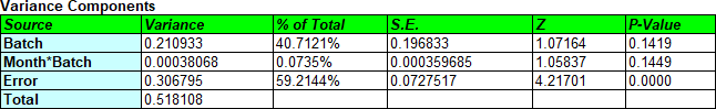
The resulting model is a single line that applies to all batches.

For the sample data, this results in the longest shelf life yet. It also results in much better residuals.

Of course, we must be wary of John Tukey's warning against data snooping (trying lots of models until we find one that gives us the answers that we want). As always, it's best to have a modeling protocol in place before you look at the data. Still, when establishing that protocol it can be helpful to compare different approaches.

Webinar

For more information, view our recorded webinar.

References

• Chow, S. (2007). Statistical Design and Analysis of Stability Studies.
• U.S. Department of Health and Human Services, Food and Drug Administration, (2003). Guidance for Industry, Q1A(R2) Stability Testing of New Drug Substances and Products.
• U.S. Department of Health and Human Services, Food and Drug Administration, (2004). Guidance for Industry, Q1E Evaluation of Stability Data.