
Many types of data are collected over time. Stock prices, sales volumes, interest rates, and quality measurements are typical examples. Because of the sequential nature of the data, special statistical techniques that account for the dynamic nature of the data are required. Statgraphics' products provides several procedures for dealing with time series data:

| Procedure | Statgraphics Centurion 18/19 | Statgraphics Sigma express |
Statgraphics stratus |
Statgraphics Web Services |
StatBeans |
|---|---|---|---|---|---|
| Run Charts |  |
|
|||
| Baseline Plot | |
||||
| Descriptive Methods | |
|
|
|
|
| Andrews Plot | |
||||
| Open-High-Low-Close Plot | |
||||
| Smoothing | |
|
|
|
|
| Seasonal Decomposition | |
|
|
|
|
| X-13-ARIMA-SEATS | |
||||
| Forecasting (User-Specified Model) | |
|
|
|
|
| Forecasting (Automatic Model Selection) | |
|
|
||
| Exponential Smoothing | |
The Run Chart procedure plots data contained in a single numeric column. It is assumed that the data are sequential in nature, consisting either of individuals (one measurement taken at each time period) or subgroups (groups of measurements at each time period). Tests are performed on the data to determine whether they represent a random series, or whether there is evidence of mixing, clustering, oscillation, or trending.

More:Run Chart.pdf
Characterizing a time series involves estimating not only a mean and standard deviation but also the correlations between observations separated in time. Tools such as the autocorrelation function are important for displaying the manner in which the past continues to affect the future. Other tools, such as the periodogram, are useful when the data contain oscillations at specific frequencies.

More:Time Series - Descriptive Methods.pdf

This procedure plots a time series in sequential order, identifying points that are beyond lower and/or upper limits. It is widely used to plot monthly data such as the Oceanic Niño Index.

More: Time Series Baseline Plot.pdf or Watch Video
Open-High-Low-Close Candlestick Plot
The Open-High-Low-Close Candlestick Plot Statlet is designed to plot security prices in a manner often used by stock traders. It shows the opening price for each trading session, high and low prices during the session, and the closing price using a graphical image often referred to as a candlestick. Trading volumes may also be displayed as bars along the bottom of the plot.

More: Open-High-Low-Close Candlestick Plot.pdf
When a time series contains a large amount of noise, it can be difficult to visualize any underlying trend. Various linear and nonlinear smoothers may be used to separate the signal from the noise.

When the data contain a strong seasonal effect, it is often helpful to separate the seasonality from the other components in the time series. This enables one to estimate the seasonal patterns and to generate seasonally adjusted data.

More:Seasonal Decomposition.pdf
The X-13ARIMA-SEATS Seasonal Adjustment performs a seasonal adjustment of time series data using the procedure currently employed by the United States Census Bureau.

More: Seasonal Adjustment using X-13ARIMA-SEATS.pdf or Watch Video
A common goal of time series analysis is extrapolating past behavior into the future. The STATGRAPHICS forecasting procedures include random walks, moving averages, trend models, simple, linear, quadratic, and seasonal exponential smoothing, and ARIMA parametric time series models. Users may compare various models by withholding samples at the end of the time series for validation purposes.

More: Forecasting.pdf
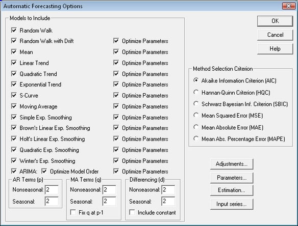
If desired, users may elect to let STATGRAPHICS select a forecasting model for them by comparing multiple models and automatically picking the model that maximizes a specified information criterion. The available criteria are based on the mean squared forecast error, penalized for the number of model parameters that must be estimated from the data. A common use of this procedure in Six Sigma is to select an ARIMA model on which to base an ARIMA control chart, which unlike most control charts does not assume independence between successive measurements. In such cases, the analyst may elect to consider only models of the ARMA(p,p-1) form, which theory suggests can characterize many dynamic processes.
More: Automatic Forecasting.pdf
This Statlet applies various types of exponential smoothers to a time series. It generates forecasts with associated forecast limits. Using the Statlet controls, the user may interactively change the values of the smoothing parameters to examine their effect on the forecasts.

More: Exponential Smoothing Statlet.pdf


© 2025 Statgraphics Technologies, Inc.
The Plains, Virginia
CONTACT US
Have you purchased Statgraphics Centurion or Sigma Express and need to download your copy?
CLICK HERE


